My "A trous" wavelet library with Python 2 bindings, which can be used to filter 1-D, 2-D and 3-D arrays.
There are a few (hopefully useful) tricks I have implemented in the library:
In [1]:
import libatrous
import numpy as np
%matplotlib inline
import matplotlib as mpl
import matplotlib.pyplot as plt
mpl.rcParams['figure.figsize'] = (20.0, 20.0)
import scipy.misc
In [2]:
kernel_names = libatrous.get_names()
print kernel_names
In [3]:
kernel = libatrous.get_kernel(0)
kernel
Out[3]:
Calculating the individual scales and residual low pass is an iterative process. For this, only one (optimised) function is required:
libatrous.iterscale(lowpass, kernel, scale_index)
With large input arrays, the memory required to store every single scale (and residual) can quickly become an issue, especially since we are malloc-ating the required memory as a contiguous block of memory (don't do that!).
Here is how we would use libatrous.iterscale to create a python list of arrays, where only the individual scales (and residual) are contiguous, not the total amount of memory required to store the array. This is only marginally better, but may not overflow the system if a contiguous block cannot be allocated.
The scenario for this is when we want to pre-compute a bunch of scales, up to a pre-defined largest scale (slow), and then interactively add any of the scales and / or residual together to generate the output array (fast).
In [4]:
def get_scales(input_array, nscales, kernel):
scales = []
lowpass = input_array.astype(np.float32)
for i in range(nscales):
bandpass,lowpass = libatrous.iterscale(lowpass,kernel,i)
scales.append(bandpass)
scales.append(lowpass)
return scales
However, we often only need the resulting band pass filter between scale1 and scale2 (0-indexed, scale2 excluded), in which case there is no need to allocate memory for the individual scales, only for the output image.
In [5]:
def get_bandpass(input_array, scale1, scale2, kernel, lowpass = False):
output = np.zeros(input_array.shape, np.float32)
lowpass = input_array.astype(np.float32)
for i in range(scale2+1):
bandpass,lowpass = libatrous.iterscale(lowpass,kernel,i)
if i >= scale1:
output += bandpass
if lowpass:
output += lowpass
return output
Finally, in some cases, we may only be interested in the low-pass residual, after having discarded N scales.
In [6]:
def get_lowpass(input_array, n_discarded, kernel):
lowpass = input_array.astype(np.float32)
for i in range(n_discarded):
bandpass,lowpass = libatrous.iterscale(lowpass,kernel,i)
return lowpass
In [7]:
def display_scales(title,scales,limits=None):
if limits is None:
nx1,nx2 = 0,scales[0].shape[1]
ny1,ny2 = 0,scales[0].shape[0]
else:
nx1,nx2,ny1,ny2 = limits
nscales = len(scales)
mpl.rcParams['figure.figsize'] = (20.0, 20.0)
fig, subplots = plt.subplots(1,nscales)
for i in range(nscales):
if i == nscales-1:
title = "Low-pass residual"
elif i > 0:
title = "Scale %d" % (i)
ax = subplots[i]
ax.imshow(scales[i][ny1:ny2,nx1:nx2],cmap='gray')
ax.set_axis_off()
ax.set_title(title)
In [8]:
nscales = 4
kernel_names = libatrous.get_names()
n_kernel = len(kernel_names)
ascent = scipy.misc.ascent()
for j in range(n_kernel):
kernel = libatrous.get_kernel(j)
print("Kernel %s coefficients: %s" % (kernel_names[j],str(kernel)))
scales = [ascent]+get_scales(ascent,nscales,kernel)
display_scales(kernel_names[j],scales)
By using separable kernels, input arrays can in principle be of any dimension. However, only 1-D, 2-D and 3-D arrays are recognised for now.
When using libatrous to filter 3-D microscopy images, voxels often do not have the same dimension in X,Y and Z. This needs to be accounted for to avoid over-emphasising any of the X,Y or Z directions.
Voxel dimensions are input using the following command (for a 0.24,0.24,1.00um voxel):
In [9]:
libatrous.set_grid(0.24,0.24,1)
This is done during calculations by considering the (equivalent) nearest neigbour at the requested position.
Also, when working with 2-D+time stacks, we may want to either apply a filter in the Z (time) direction only, or apply the filter in the X and Y directions for each frame in the stack but not apply the filter in the Z direction.
I added the enable_conv() function to control which dimensions the separable filter kernel is applied to.
In the first case and before applying the filter, use:
In [10]:
libatrous.enable_conv(0,0,1)
And in the second case:
In [11]:
libatrous.enable_conv(1,1,0)
In [12]:
nscales = 4
ascent = scipy.misc.ascent()
ny,nx = ascent.shape
scales = [ascent]
ascent = np.tile(ascent,(16,16))
print("Image size: %s" % str(ascent.shape))
In [13]:
import pywt
import time
factor=1
cdf97_an_lo = factor*np.array([0, 0.026748757411, -0.016864118443, -0.078223266529, 0.266864118443,\
0.602949018236, 0.266864118443, -0.078223266529,-0.016864118443, \
0.026748757411])
cdf97_an_hi = factor*np.array([0, 0.091271763114, -0.057543526229,-0.591271763114,1.11508705,\
-0.591271763114,-0.057543526229,0.091271763114,0, 0 ])
cdf97_syn_lo = factor*np.array([0, -0.091271763114,-0.057543526229,0.591271763114,1.11508705,\
0.591271763114 ,-0.057543526229,-0.091271763114,0, 0])
cdf97_syn_hi = factor*np.array([0, 0.026748757411,0.016864118443,-0.078223266529,-0.266864118443,\
0.602949018236,-0.266864118443,-0.078223266529,0.016864118443,\
0.026748757411])
cdf97 = pywt.Wavelet('cdf97', [cdf97_an_lo,cdf97_an_hi,cdf97_syn_lo,cdf97_syn_hi])
In [14]:
t = time.time()
result = pywt.swt2(ascent, cdf97, level=nscales, start_level=0)
print("Took: %.2fs" % (time.time()-t))
LL_old = ascent
for LL, (LH, HL, HH) in result:
HH_ = LL_old-LL
LL_old = LL
scales.append(HH_)
scales.append(LL)
display_scales("CDF 9/7 (pywt)",scales,(0,nx,0,ny))
del result,scales
In [15]:
scales = [ascent]
kernel = libatrous.get_kernel(4)
#Use all the cores...
libatrous.set_ncores(24)
t = time.time()
scales += get_scales(ascent,nscales,kernel)
print("Took: %.2fs" % (time.time()-t))
display_scales("CDF 9/7 (libatrous)",scales,(0,nx,0,ny))
del scales
libatrous.set_ncores() can be used to limit the number of cores allocated by OpenMP.
This is useful when libatrous is used in threads instanciated from Python (e.g. CellProfiler), in which case, reducing the number of threads allocated by libatrous to 1 may actually speed things up.
Here we look at the increase in speed with number of cores, compared to the time it takes to process the image with a single core:
In [16]:
max_cores = 15
ascent = scipy.misc.ascent()
ascent = np.tile(ascent,(16,16))
cores = np.zeros(max_cores)
ts = np.zeros(max_cores)
speed = np.zeros(max_cores)
for i in range(max_cores):
libatrous.set_ncores(i+1)
t = time.time()
scales = get_scales(ascent,nscales,kernel)
ts[i] = time.time()-t
cores[i] = i+1
if i == 0:
speed[i] = 1
else:
speed[i] = ts[0]/ts[i]
mpl.rcParams['figure.figsize'] = (10.0, 10.0)
fig, ax = plt.subplots(1,1)
ax.plot(cores,ts,'b-')
ax.set_xlabel("Number of allocated cores")
ax.set_ylabel("Time to process (s)")
ax.tick_params('y', colors='b')
ax2 = ax.twinx()
ax2.plot(cores,speed,'r-')
ax2.set_ylabel("Speed factor")
ax2.tick_params('y', colors='r')
ax.set_title("(%d,%d) image array split into %d scales + lp residual" % (ascent.shape[0],ascent.shape[1],nscales))
_ = ax.set_xlim(1,max_cores)
my implementation closely matches [1], however I changed my edge stopping function to fit with the separable kernel calculation strategy, as per [2].
Basically equation (3) in [1],
\begin{align} G_{\sigma_r} ( a^i_m - a^i_n) = exp \left( - \frac{\|a^i_m - a^i_n\|^2}{\sigma_r^2}\right) \\ \end{align}is replaced by
\begin{align} G_{\sigma_r} ( a^i_m - a^i_n) = exp \left( - \frac{\|a^i_m - a^i_n\|}{\sigma_r}\right) \\ \end{align}according to the code described in [2] and applied for each dimension as part of the kernel convolution calculation. The normalisation factor $W_a$ in equation (4) is also calculated and applied separately for each dimension.
Be aware in [1] that $\sigma_r$ is a fraction of the max value of the input image (as far as I understand).
$\alpha$ is the shrinkage rate of $\sigma_r$.
Also, [1] uses the B3 Spline 5x5 kernel coefficients, as in libatrous.get_kernel(1).
Let's modify the previous iterative scale calculation to add the stopping function and use an optimised libatrous function that applies it and the shrinkage rate. The new get_scales_ea() takes the following arguments:
At each step, the stopping function map (dmap) is calculated by get_dmap() for intensity differences between 0 and max_input. To calculate dmap, the 0-indexed scale, number of scales, sigmar, alpha and max_input need to be passed as parameters.
In [17]:
def get_scales_ea(input_array, nscales, kernel, sigmar, alpha):
scales = []
max_input = int(np.amax(input_array))
sigmar = sigmar * max_input
lowpass = input_array.astype(np.float32)
for i in range(nscales):
dmap = libatrous.get_dmap(i,nscales,sigmar,alpha,max_input)
bandpass,lowpass = libatrous.iterscale_ea(lowpass,kernel,dmap,i)
scales.append(bandpass)
scales.append(lowpass)
return scales
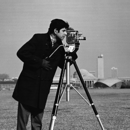
Let's try with the cameraman picture as in [1].
In [18]:
import scipy.ndimage
cameraman = scipy.ndimage.imread("cameraman.png")
print cameraman.shape
In [19]:
nscales = 5
kernel_names = libatrous.get_names()
n_kernel = len(kernel_names)
sigmar = 0.2
alpha = 2
for j in range(n_kernel):
kernel = libatrous.get_kernel(j)
scales = [cameraman]+get_scales_ea(cameraman,nscales,kernel,sigmar,alpha)
display_scales(kernel_names[j],scales,(128,178,160,210))
In [20]:
fig, subplots = plt.subplots(1,2)
ax = subplots[0]
ax.imshow(cameraman,cmap='gray')
ax.set_axis_off()
ax.set_title("Input")
ax = subplots[1]
ax.imshow(scales[-1],cmap='gray')
ax.set_axis_off()
_ = ax.set_title("Residual low-pass after subtracting %d scales (%s)" % (nscales,kernel_names[-1]))
In [ ]: