Linear Regression Lab February 17th 2015

Regression refers to the technique employed when learning a mapping from vector of input data to a quantitative output. For example, coordinates in a room to temperature, someone's Body Mass Index to their life expectancy or a stock's performance over the last 5 days to it's value tomorrow.

There are numerous methods for addressing this problem, each with their own set of assumptions and behaviour. Some are ideal for tackling large volumes of data while others provide more informative probabilistic outputs.

In this lab, we'll focus on Linear Regression; a good point of reference for many other regression techniques and still used widely around the world today due to their simplicity and favourable scaling characteristics.

Part I: Maximum Likelihood Linear Regression

In this section, we're going to explore what linear regression models are and investigate how they can be trained using a "Maximum Likelihood" approach.

First, lets generate some synthetic data. Here's we create a random 1-D vector $\mathbf{x}$ of observation locations and evaluate an "unknown" ground truth function at these locations before adding some noise to create our observations, $\mathbf{y}$.

Lets plot the data first to see what it looks like:

Linear Model with Polynomial Features

Okay, now lets try to fit a model to it.

One of the most straightforward types of regression is maximum likelihood regression using a linear model, (the output is a weighted sum of the features). For now, lets use a very simple model with just two parameters (or weights), $\mathbf{w}$. \begin{equation} f(x) = w_0 + w_1 x \end{equation} In matrix form this is $\mathbf{f}= \mathbf{\theta w}$ where $\mathbf{\theta}$ is $[x^0,x^1]$ (the feature matrix) and $\mathbf{w}$ is $[w_0, w_1]^T$.

The feature matrix has a dimensionality of $N\times p$ where $N$ is the number of inputs and $p$ is the number of features. The complexity of the model can be increased by increasing $p$. Polynomial features (increasing powers of $x$) are commonly used in practice. Evaluating a polynomial model at locations $[x_1,...,x_N]$ and weights $[w_0,...,w_p]$ is given as:

\begin{equation} \begin{bmatrix} f_1 \\ f_2 \\ \vdots \\ f_N \end{bmatrix} = \begin{bmatrix} x_1^0 & x_1^1 & \cdots & x_1^{p-1} \\ x_2^0 & x_2^1 & \cdots & x_2^{p-1} \\ \vdots & \vdots & \ddots & \vdots \\ x_N^0 & x_N^1 & \cdots & x_N^{p-1} \end{bmatrix} \begin{bmatrix} w_0 \\ w_1 \\ \vdots \\ w_{p-1} \end{bmatrix} \end{equation}

Lets query our model and compare it against the data. To generate a polynomial feature matrix $\theta$, we'll use a custom function called polyFeatureGen() that takes the observation or query locations ($x$ or $x_{\text{query}}$) and the number of features ($p$) as inputs. It returns an $n \times p$ matrix such that: \begin{equation} \theta_{i,j} = x_i^{j-1} \end{equation}

Complete the function in the cell below:

For now, lets stick with two features. Lets pick two arbitriary values for the weights. Say,

Generate the query points and the associated feature matrix

Write a line of code to generate the associated feature matrix for the query points:

Now evaluate the model at the query locations by multiplying the query feature matrix by our guessed weights:

And plot the results:

It's not a great fit! The Mean Squared Error between the model predictions and the observations is:

Maximum Likeliood Estimation

Now lets learn the parameters of our model to see if we can improve the fit. The goal here is to estimate the parameter values (i.e. $\mathbf{w}$) from the data. A popular way of doing this is by maximising the conditional likelihood of the data given a model, $p(y|x,w,\beta^{-1})$, with respect to the parameters.

A common assumption to make is that the measurements we gathered are subject to Gaussian noise i.e. we assume that our observations, y are drawn from a Gaussian distribution with mean $\mathbf{w\theta^T}$ and variance $\beta^{-1}$ (indicating the level of noise).

The probability of acquiring a particular set of observation, given a specific model is \begin{equation} p(y|x,w,\beta^{-1}) = \prod_{n=1}^{N} \mathcal{N}(\mathbf{w\theta^T}, \beta^{-1}) \end{equation}

It is often referred to as the likelihood of the data. In log form: \begin{equation} \text{ln}p(\mathbf{y}|\mathbf{x},\mathbf{w},\beta^{-1}) = \sum_{n=1}^{N} \text{ln}\big( \mathcal{N}(\mathbf{w\theta^T}, \beta^{-1})\big) \\ = \frac{N}{2} \text{ln}(\beta) - \frac{N}{2}\text{ln}(2\pi) - \frac{\beta}{2} \sum_{n=1}^{N} (\mathbf{y}-\mathbf{w\theta^T})^2 \end{equation}

The final term is the sum of squares error between the observations and the model. If we vary the parameters of the model to maximise the likelihood of the data, we train a model that best fits the data The gradient of the log likelihood with respect to the weights is: \begin{equation} \triangledown \text{ln}p(\mathbf{y}|\mathbf{x},\mathbf{w},\beta^{-1})= \sum_{n=1}^{N} (\mathbf{y}_n - \mathbf{w\theta^T})\theta \end{equation} Find the max by setting the gradient to zero and then solve for $\mathbf{w}$ to find the "maximum-likelihood parameters" (wml): \begin{equation} \mathbf{w}{ml}^T = (\mathbf{\theta}^T\mathbf{\theta})^{-1}\mathbf{\theta^T y} \end{equation}

Generate the feature matrix using the observations locations.

Then find the parameters that maximise the likelihood as described above.

Now evaluate the model at the query locations using the new parameters and plot the raw data and the new model's prediction as before:

Much better. Calculate and print the mean squared error between the model predictions and the observations using these new parameters to quantively compare with our initial set of parameters:

This MSE is the best we can do with this model.

Increasing the Model Complexity

To reduce the MSE further, we will need to increase the model's flexibility by adding higher order polynomial features. In the cell below, change the number of features in the model. Run the cell to learn the max likelihood weights for that set of features, plot the resulting query outputs as before and evaluate the MSE. What is the number of features that gives the lowest MSE?

As you may have noticed, increasing the flexibility and model complexity decreases the mean squared error because the model's ability to fit all of the observation exactly increases as well. However, it also results in "overfitting". This is when the model fits the observations very well but generalises poorly to out locations. If a number of observations are withheld from training, the model would not do well at predicting their value as it is more concerned with overfitting the observations it can see.

Basis Functions

Up until now, the feature matrix has been generated using polynomial equation:

\begin{equation} \theta_{i,j} = x_i^{j-1} \end{equation}

This is sometimes referred to as the polynomial basis function.

Run the cell below to visualise the basis functions that were used in the last model you trained:

The above graph is simply plotting each column or feature of the feature matrix. Uncomment and complete the line of code in the cell below to plot the basis functions multipled by their associated learnt weight.

Interestingly, the model's complicated looking prediction is just a linear combination of these basis functions. Hence the name "linear" regression.

There are many possible variants of basis functions each giving the resulting model different characteristics (e.g. smooth, non-stationary, discontinuous etc.).

Radial basis functions are a commonly used alternative to the polynomial function: \begin{equation} \theta_{i,j} = \text{exp}\Bigg(-\frac{(x_i-\mu_j)^2}{2s^2}\Bigg) \end{equation} Here, $\mu_j$, is the mean of the $j^{\text{th}}$ radial basis function and $s$ corresponds to the basis functions width or its region of influence.

Implement the basis function radialFeatureGen() that takes a vector of inputs ($\textbf{x}$), a vector of $p$ mean locations ($\mathbf{\mu}$) with shape $p \times 1$ and a basis function spatial width ($s$). It then calculates the feature matrix, $\theta$, using the radial basis function given above.

Using the values for $\mu$ and $s$ provided below, write some code that finds the weights with the maximum likelihood ($w_{ml}$) for a design matrix generated using the radial basis function. Then evaluate the model at the query locations and plot the results as before.

Rerun the above cell but change the basis functions by altering $\mu$. e.g. mu = np.array([1,2,3,4,5,6,7,8,9,10])[:,np.newaxis]

• What effect does changing $s$ have on the model?
• How might we find the optimal values for $\mu$ and $s$?
• How does the behaviour of the radial basis function model differ from the polynomial case in regions far from data?

Downsides to Maximum Likelihood Regression

While this approach to regressing over data is appealling, it does have a few shortcomings. For example, we have no estimate of how confident the model is in its predictions (which can be crucial in decision-making applications). Also the model learns a single hypothesis to explain the data. In reality there may be numerous explanations for the same set of observations. In Part II of today's lab, we will investigate a probabilitic approach to regression.

$$ % Bayesian Linear Regression Tutorial, Alistair Reid, NICTA 2015 \newcommand{\W} [0] {\mathbf{w}} \newcommand{\X} [0] {\mathbf{x}} \newcommand{\y} [0] {\mathbf{y}} \newcommand{\Xf} [0] {\mathbf{\theta}} \newcommand{\norm} [0] {\mathcal{N}} \newcommand{\weightprec} [0] {Q} \newcommand{\weightprecsimp} [0] {\alpha I} \newcommand{\alphs} [0] {\mathbf{\alpha}} \newcommand{\invnoise} [0] {\beta} \newcommand{\noise} [0] {\beta^{-1}} \newcommand{\Ainv} [0] {A^{-1}} \newcommand{\fq} [0] {\mathbf{f_*}} \newcommand{\xq} [0] {\mathbf{x_*}} $$

Part 2: Bayesian Linear Regression

In the previous sections, we have selected the linear regression weights by maximising the likelihood of the data. The learnt model certainly makes useful predictions, but it provides no notion of uncertainty: we cannot distinguish between a prediction that is tightly constrained by the data, and a prediction that is essentially an unconstrained `guess'. Also, if there are multiple likely explanations of the data, we have neglected all but one. Recall that for a given feature mapping $\X \to \Xf$, the predictive behaviour of a linear regression is encoded in the weights: \begin{equation} f(x) = \Xf \W \end{equation}

Where $\W$ is $p \times 1$ and $\Xf$ is $n \times p$. Instead of using a single maximum likelihood weight vector, we can take a Bayesian approach and consider a probability distribution over all possible weight vectors. The distribution can be inferred from the observations using Bayes rule:

\begin{equation} p(\W|\y) \propto p(\y|\W) p(\W) \end{equation}

The likelihood $p(\y|\W)$ is exactly the criterion we were using to select the maximum likelihood weights:

\begin{equation} p(\y | \W) = \norm (y | \Xf \W, \noise I ) \end{equation}

In addition, we must now specify a prior distribution over $\W$ encoding our belief about reasonable weight values. Any probability distribution we consider to be sensible for the problem could be used here, but some are easier to work with than others. In this tutorial, we will use a simple Gaussian prior with precision (inverse covariance) $\weightprecsimp$ that is $p \times p$ with a single free parameter:

\begin{equation} \W \sim \norm( 0, \alphs^{-1}I ) \end{equation}

Hence we are assuming the weights are independently distributed & penalised for large magnitudes. While the $\W$'s are model parameters that directly affect the output, we consider the $\alphs$'s to be hyperparameters because they tune the prior distribution over the parameters $\W$.

Because we have assumed a Gaussian form for both the likelihood and the prior, Bayes rule can be computed analytically in this case to obtain a posterior distribution over the weights. This involves expanding the exponents of the two Gaussians and completing the square (an exercise left to the reader).

The posterior over the weights is given by: \begin{equation} p(\W|\Xf,y) \sim \norm \left( \mu_w, \Ainv \right) \end{equation} Where $A$ is the $p \times p$ posterior precision given by: \begin{equation} A = \invnoise \Xf^\top \Xf + \weightprecsimp \end{equation} And the weight means are given by: \begin{equation} \mu_w = \invnoise \Ainv \Xf^\top \y \end{equation}

Exercise: Compute Posterior Weight Distribution

Add some code to compute $A$ and $\mu_w$ in the cell below:

Marginalising over weights

While it is interesting to see the distribution of weights used by the Bayesian linear regression, the ultimate goal is to predict the outputs $\fq$ corresponding to inputs $\xq$. To do this, we marginalise out the weights $\W$:

\begin{equation} p(\fq | \xq, \Xf, \y) = \int p(\fq|\xq,\W) p(\W|\Xf,\y) d\W \end{equation}

We know from above that: \begin{equation} p(\W|\Xf,y) \sim \norm ( \mu_w, \Ainv ) \end{equation}

We have also defined a deterministic mapping to the predictive function: \begin{equation} \fq = \xq \W \end{equation}

This marginalisation has a closed form solution - we can produce predictive distributions, considering all possible weights, without explicity computing them: \begin{equation} \fq \sim \norm \left( \invnoise \xq \Ainv \Xf^\top \y, \hspace{0.5cm} \xq \Ainv \xq^\top \right) \end{equation}

Note that this equation gives a multivariate Gaussian prediction: for $m$ queries, the covariance will be $m \times m$. This is useful for joint draws. However, if you are only interested in the envelope of uncertainty, then the diagonal can be extracted to give the marginal variance of each prediction. Don't forget to add the noise variance back on if you want to predict the range of possible observations rather than latent functions!

Exercise:

Complete the unfinished lines of code in the cell below:

Exercise: Non-linear Basis Functions

We have already been using simple linear basis functions, but lets try a demo with a non-linear problem. Don't worry about visualising the distribution over weights - with many polynomial features they will be too high dimensional to show, but we will get very interesting predictive marginals:

This data clearly has a non-linear pattern. As we saw in part 1 of this tutorial, linear regression techniques can perform well on non-linear data by introducing basis functions. Lets apply the polynomial basis functions you implemented in polyFeatureGen to increase the dimensionality of the inputs to $p=7$ and run the regression again.

Complete the unfinished lines of code in the cell below:

Now the predictions are able to capture the non-linear structure of this problem! There are two ways of interpreting how this is working.

The first interpretation is that we are inferring a probability distribution over the weights, and each weight corresponds to a basis function. With the polynomial basis functions, we are therefore considering distributions over the polynomial coefficients in a polynomial equation. You can see in the predictive distribution: \begin{equation} \fq \sim \norm \left( \invnoise \xq \Ainv \Xf^\top \y, \hspace{0.5cm} \xq \Ainv \xq^\top \right) \end{equation} that our mean function is in fact a linear combination of the basis functions composing $\Xf$, and the space of models is restricted to the span of the basis functions.

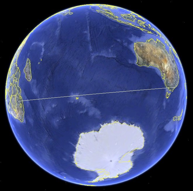
A second interpretation is that we have used polyFeatureGen to project the inputs and the queries into 7 dimensions, effectively warping the space on the x-axis. The line in the high dimensional space can then project to a nonlinear function in the original space. To understand this principle, think about how a direct path an airline takes around a 3D sphere can appear as a curved arc when projected onto a 2d map ). You will see this principle applied in the support vector machine tutorial.

You can investigate the choice of basis functions by modifying the above code:

• What happens to the prediction as you move away from the input data? (try changing the domain above)
• We have been using polynomial basis functions. Can you think of a different class of basis functions that might work for periodic data?

Plotting draws from the posterior

We have been looking at the mean and envelope of the predictive distribution, but it is also useful to look at draws from the posterior distribution. To do this we must look at the joint multivariate distribution of the posterior. Note that given our particular choice of Gaussian prior and likelihood, the posterior predictions are also joint-Gaussian. For example, we can compute a posterior multivariate Gaussian over the weights and draw random weights out of this distribution. This will sample a set of deterministic models each drawn with probability consistent with our Bayesian analysis.

How do we draw values out of a multivariate Gaussian distribution? We can do this by linear operations on a vector of independent univariate Gaussian draws. This can be achieved using the cholesky factorisation: if $L$ is the upper Cholesky factor of the covariance matrix $A^{-1}$, and $\mathbf{\Sigma}$ is a vector of iid Gaussians, we may draw from the distribution according to: \begin{equation} \hat{\W} = \mu_w + L \Sigma \end{equation}

Complete the unfinished lines of code in the cell below:

• If we were to average over a very large number of these draws, the density at each input value would be Gaussian distributed with the marginals from the previous section.

Advanced: Hyperparameter selection

Until now we have been manually specifying values for $\alphs^2$ and $\invnoise$. Such manual selection is not ideal, as it requires a deep understanding of every dataset and large amounts of manual tuning to select appropriate noise and prior hyperparameters. Instead, there are two main approaches for hyperparameter selection based on the data. Both rely on the concept of marginal likelihood - the probability of drawing the observations out of the prior. We can obtain this criterion by marginalising over the actual weight vectors and the noise draws. The log marginal likelihood given all our Gausianity assumptions so far is given by:

\begin{equation} \log p(y | \Xf) = \frac{1}{2} \left( p \log \alphs^2 + n \log \invnoise - \log |A| - n \log 2\pi - \invnoise (y-y^*)^\top (y-y^*) - \alphs^2 \mu^{*\top} \mu^* \right) \end{equation}\begin{equation} \mu^* = \invnoise \Ainv \Xf^T y \end{equation}\begin{equation} \y^* = \Xf \mu^* \end{equation}

See "Evaluation of the evidence function" in Bishop - Pattern recognition and machine learning for how this is derived. Here $|A|$ is the determinant of $A$, and $\mu^*$ and $\y^*$ are the mean weights and mean latent function predictions at $\X$ respectively using the current hyperparameters. This criterion naturally weights model fit against complexity. If the prior is too tight to fit the data, we cannot draw the observations, but if it is too general then the probability of drawing any particular dataset is also low. It can become very small or large and is best computed in log form.

The first hyperparameter strategy is to define a hyper-prior over $\alphs$ and $\mathbf{\beta}$. If we carefully choose a conjugate prior (for our scenario this will be an inverse gamma distribution) over these parameters, then it is possible to marginalise over the hyperparameters (in the same way we marginalised the weights out of the predictive distribution) and obtain a closed form solution for the weight distribution. An interested student is directed to the above textbook for a detailed explanation. Unfortunately, this distribution will be of Student-T form rather than Gaussian, so marginalising out the weights to obtain predictions will then be an exercise in numerical integration.

A simpler approach that we will take here is to search for the maximum likelihood hyperparameters - this is also called the evidence approximation or type 2 maximum likelihood. The main drawback of this approach is that we loose a level of Bayesian inference compared to the above alternative. Also we must select these parameters via optimisation strategies and the problem is non-convex, meaning we may end up in a local optimum that is better than its neighbours but not the best set of parameters. However, it is a more principled method of model selection than manual tweaking.

Below we will use a simple gradient-free numerical optimisation procedure to find some hyperparameters:

Now try using these values in the previous sections!

Part III: Stopping Distance Assignment

Now that you know the basics of linear regression, lets apply it to a real data problem. The cell below loads a dataset of stopping distances (metres) of a car travelling at different speeds (km/h). If you were in the same car travelling at 21 km/h and you hit the brakes at a distance of 135 metres from a wall, what is the probability of you coming to a stop before hitting the wall?