This notebook was put together by [Jake Vanderplas](http://www.vanderplas.com) for UW's [Astro 599](http://www.astro.washington.edu/users/vanderplas/Astr599_2014/) course. Source and license info is on [GitHub](https://github.com/jakevdp/2014_fall_ASTR599/).
In [1]:


%run talktools.py
While the Python language is an excellent tool for general-purpose programming, with a highly readable syntax, rich and powerful data types (strings, lists, sets, dictionaries, arbitrary length integers, etc) and a very comprehensive standard library, it was not designed specifically for mathematical and scientific computing. Neither the language nor its standard library have facilities for the efficient representation of multidimensional datasets, tools for linear algebra and general matrix manipulations (an essential building block of virtually all technical computing), nor any data visualization facilities.
In particular, Python lists are very flexible containers that can be nested arbitrarily deep and which can hold any Python object in them, but they are poorly suited to represent efficiently common mathematical constructs like vectors and matrices. In contrast, much of our modern heritage of scientific computing has been built on top of libraries written in the Fortran language, which has native support for vectors and matrices as well as a library of mathematical functions that can efficiently operate on entire arrays at once.
In [2]:


import numpy as np
As mentioned above, the main object provided by numpy is a powerful array. We'll start by exploring how the numpy array differs from Python lists. We start by creating a simple list and an array with the same contents of the list:
In [3]:


lst = [10, 20, 30, 40]
arr = np.array([10, 20, 30, 40])
In [4]:


lst[0]
Out[4]:
In [5]:


arr[0]
Out[5]:
In [6]:


arr[-1]
Out[6]:
In [7]:


arr[2:]
Out[7]:
The first difference to note between lists and arrays is that arrays are homogeneous; i.e. all elements of an array must be of the same type. In contrast, lists can contain elements of arbitrary type. For example, we can change the last element in our list above to be a string:
In [8]:


lst[-1] = 'a string inside a list'
lst
Out[8]:
but the same can not be done with an array, as we get an error message:
In [9]:


arr[-1] = 'a string inside an array'
In [10]:


arr.dtype
Out[10]:
Once an array has been created, its dtype is fixed and it can only store elements of the same type. For this example where the dtype is integer, if we store a floating point number it will be automatically converted into an integer:
In [11]:


arr[-1] = 1.234
arr
Out[11]:
Above we created an array from an existing list; now let us now see other ways in which we can create arrays, which we'll illustrate next. A common need is to have an array initialized with a constant value, and very often this value is 0 or 1 (suitable as starting value for additive and multiplicative loops respectively); zeros creates arrays of all zeros, with any desired dtype:
In [12]:


np.zeros(5, dtype=float)
Out[12]:
In [13]:


np.zeros(3, dtype=int)
Out[13]:
In [14]:


np.zeros(3, dtype=complex)
Out[14]:
and similarly for ones:
In [16]:


print('5 ones:', np.ones(5))
If we want an array initialized with an arbitrary value, we can create an empty array and then use the fill method to put the value we want into the array:
In [17]:


a = np.empty(4)
a.fill(5.5)
a
Out[17]:
In [18]:


np.arange(5)
Out[18]:
and the linspace and logspace functions to create linearly and logarithmically-spaced grids respectively, with a fixed number of points and including both ends of the specified interval:
In [17]:


print("A linear grid between 0 and 1:")
print(np.linspace(0, 1, 4))
In [19]:


print("A logarithmic grid between 10**1 and 10**3:")
print(np.logspace(1, 3, 4))
Finally, it is often useful to create arrays with random numbers that follow a specific distribution. The np.random module contains a number of functions that can be used to this effect, for example this will produce an array of 5 random samples taken from a standard normal distribution (0 mean and variance 1):
In [20]:


np.random.randn(5)
Out[20]:
whereas this will also give 5 samples, but from a normal distribution with a mean of 10 and a variance of 3:
In [21]:


norm10 = np.random.normal(10, 3, 5)
norm10
Out[21]:
Above we saw how to index arrays with single numbers and slices, just like Python lists. But arrays allow for a more sophisticated kind of indexing which is very powerful: you can index an array with another array, and in particular with an array of boolean values. This is particluarly useful to extract information from an array that matches a certain condition.
Consider for example that in the array norm10 we want to replace all values above 9 with the value 0. We can do so by first finding the mask that indicates where this condition is true or false:
In [22]:


mask = norm10 > 9
mask
Out[22]:
Now that we have this mask, we can use it to either read those values or to reset them to 0:
In [24]:


print('Values above 9:', norm10[mask])
In [25]:


print('Resetting all values above 9 to 0...')
norm10[mask] = 0
print(norm10)
Up until now all our examples have used one-dimensional arrays. But Numpy can create arrays of aribtrary dimensions, and all the methods illustrated in the previous section work with more than one dimension. For example, a list of lists can be used to initialize a two dimensional array:
In [26]:


lst2 = [[1, 2], [3, 4]]
arr2 = np.array([[1, 2], [3, 4]])
arr2
Out[26]:
With two-dimensional arrays we start seeing the power of numpy: while a nested list can be indexed using repeatedly the [ ] operator, multidimensional arrays support a much more natural indexing syntax with a single [ ] and a set of indices separated by commas:
In [28]:


print(lst2[0][1])
print(arr2[0,1])
In [29]:


np.zeros((2,3))
Out[29]:
In [30]:


np.random.normal(10, 3, (2, 4))
Out[30]:
In fact, the shape of an array can be changed at any time, as long as the total number of elements is unchanged. For example, if we want a 2x4 array with numbers increasing from 0, the easiest way to create it is:
In [32]:


arr = np.arange(8).reshape(2, 4)
arr
Out[32]:
In [34]:


arr = np.arange(8)
arr2 = arr.reshape(2, 4)

arr[0] = 1000
print(arr)
print(arr2)
This lack of copying allows for very efficient vectorized operations.
In [37]:


print('Slicing in the second row:', arr2[1, 2:4])
print('All rows, third column   :', arr2[:, 2])
If you only provide one index, then you will get an array with one less dimension containing that row:
In [39]:


print('First row:  ', arr2[0])
print('Second row: ', arr2[1])
In [42]:


arr = arr2
In [43]:


print('Data type                :', arr.dtype)
print('Total number of elements :', arr.size)
print('Number of dimensions     :', arr.ndim)
print('Shape (dimensionality)   :', arr.shape)
print('Memory used (in bytes)   :', arr.nbytes)
Arrays also have many useful methods, some especially useful ones are:
In [44]:


print('Minimum and maximum             :', arr.min(), arr.max())
print('Sum and product of all elements :', arr.sum(), arr.prod())
print('Mean and standard deviation     :', arr.mean(), arr.std())
For these methods, the above operations area all computed on all the elements of the array. But for a multidimensional array, it's possible to do the computation along a single dimension, by passing the axis parameter; for example:
In [45]:


print('For the following array:\n', arr)
print('The sum of elements along the rows is    :', arr.sum(axis=1))
print('The sum of elements along the columns is :', arr.sum(axis=0))
As you can see in this example, the value of the axis parameter is the dimension which will be consumed once the operation has been carried out. This is why to sum along the rows we use axis=0.
This can be easily illustrated with an example that has more dimensions; we create an array with 4 dimensions and shape (3,4,5,6) and sum along the axis number 2 (i.e. the third axis, since in Python all counts are 0-based). That consumes the dimension whose length was 5, leaving us with a new array that has shape (3,4,6):
In [46]:


np.zeros((3,4,5,6)).sum(2).shape
Out[46]:
Another widely used property of arrays is the .T attribute, which allows you to access the transpose of the array:
In [48]:


print('Array:\n', arr)
print('Transpose:\n', arr.T)
We don't have time here to look at all the methods and properties of arrays, here's a complete list. Simply try exploring some of these IPython to learn more, or read their description in the full Numpy documentation:
arr.T             arr.copy          arr.getfield      arr.put           arr.squeeze
arr.all           arr.ctypes        arr.imag          arr.ravel         arr.std
arr.any           arr.cumprod       arr.item          arr.real          arr.strides
arr.argmax        arr.cumsum        arr.itemset       arr.repeat        arr.sum
arr.argmin        arr.data          arr.itemsize      arr.reshape       arr.swapaxes
arr.argsort       arr.diagonal      arr.max           arr.resize        arr.take
arr.astype        arr.dot           arr.mean          arr.round         arr.tofile
arr.base          arr.dtype         arr.min           arr.searchsorted  arr.tolist
arr.byteswap      arr.dump          arr.nbytes        arr.setasflat     arr.tostring
arr.choose        arr.dumps         arr.ndim          arr.setfield      arr.trace
arr.clip          arr.fill          arr.newbyteorder  arr.setflags      arr.transpose
arr.compress      arr.flags         arr.nonzero       arr.shape         arr.var
arr.conj          arr.flat          arr.prod          arr.size          arr.view
arr.conjugate arr.flatten arr.ptp arr.sort Arrays support all regular arithmetic operators, and the numpy library also contains a complete collection of basic mathematical functions that operate on arrays. It is important to remember that in general, all operations with arrays are applied element-wise, i.e., are applied to all the elements of the array at the same time. Consider for example:
In [50]:


arr1 = np.arange(4)
arr2 = np.arange(10, 14)
print(arr1, '+', arr2, '=', arr1+arr2)
Importantly, you must remember that even the multiplication operator is by default applied element-wise, it is not the matrix multiplication from linear algebra (as is the case in Matlab, for example):
In [51]:


print(arr1, '*', arr2, '=', arr1*arr2)
We may also multiply an array by a scalar:
In [52]:


1.5 * arr1
Out[52]:
This is a first example of broadcasting
In [53]:


print(np.arange(3))
print(np.arange(3) + 5)
We can also broadcast a 1D array to a 2D array, in this case adding a vector to all rows of a matrix:
In [54]:


np.ones((3, 3)) + np.arange(3)
Out[54]:
We can also broadcast in two directions at a time:
In [55]:


np.arange(3).reshape((3, 1)) + np.arange(3)
Out[55]:
Broadcasting rules can do the following:
If the two arrays differ in their number of dimensions, the shape of the array with fewer dimensions is padded with ones on its leading (left) side.
If the shape of the two arrays does not match in any dimension, the array with shape equal to 1 in that dimension is stretched to match the other shape.
If in any dimension the sizes disagree and neither is equal to 1, an error is raised.
Note that all of this happens without ever actually creating the stretched arrays in memory! This broadcasting behavior is in practice enormously powerful, especially because when numpy broadcasts to create new dimensions or to 'stretch' existing ones, it doesn't actually replicate the data. In the example above the operation is carried as if the 1.5 was a 1-d array with 1.5 in all of its entries, but no actual array was ever created. This can save lots of memory in cases when the arrays in question are large and can have significant performance implications.
So when we do
np.arange(3) + 5
The scalar 5 is
After these two operations are complete, the addition can proceed as now both operands are one-dimensional arrays of length 3.
When we do
np.ones((3, 3)) + np.arange(3)
The second array is
When we do
np.arange(3).reshape((3, 1)) + np.arange(3)
Then the operation proceeds as if on two 3 $\times$ 3 arrays
The general rule is: when operating on two arrays, NumPy compares their shapes element-wise. It starts with the trailing dimensions, and works its way forward, creating dimensions of length 1 as needed. Two dimensions are considered compatible when
If these conditions are not met, a ValueError: frames are not aligned exception is thrown, indicating that the arrays have incompatible shapes. The size of the resulting array is the maximum size along each dimension of the input arrays.
In [56]:


arr1 = np.ones((2, 3))
arr2 = np.ones((2, 1))

arr1 + arr2
Out[56]:
In [57]:


arr1 = np.ones((2, 3))
arr2 = np.ones(2)

arr1 + arr2
In [58]:


arr1 = np.ones((2, 3))
arr2 = np.ones((2, 1))

arr1 + arr2
Out[58]:
In [58]:
In [59]:


A = np.arange(1, 9).reshape((2, 4))
B = np.arange(1, 3)
A + B.reshape((2, 1))
Out[59]:
Another way to change the shape of B is to use the newaxis keyword:
In [61]:


print(B.shape)
print(B[:, np.newaxis].shape)
In [62]:


A + B[:, np.newaxis]
Out[62]:
As we mentioned before, Numpy ships with a full complement of mathematical functions that work on entire arrays, including logarithms, exponentials, trigonometric and hyperbolic trigonometric functions, etc. Furthermore, scipy ships a rich special function library in the scipy.special module that includes Bessel, Airy, Fresnel, Laguerre and other classical special functions. For example, sampling the sine function at 100 points between $0$ and $2\pi$ is as simple as:
In [63]:


x = np.linspace(0, 2*np.pi, 100)
y = np.sin(x)
Numpy ships with a basic linear algebra library, and all arrays have a dot method whose behavior is that of the scalar dot product when its arguments are vectors (one-dimensional arrays) and the traditional matrix multiplication when one or both of its arguments are two-dimensional arrays:
In [65]:


v1 = np.array([2, 3, 4])
v2 = np.array([1, 0, 1])

print(v1, '.', v2, '=', np.dot(v1, v2))
Here is a regular matrix-vector multiplication, note that the array v1 should be viewed as a column vector in traditional linear algebra notation; numpy makes no distinction between row and column vectors and simply verifies that the dimensions match the required rules of matrix multiplication, in this case we have a $2 \times 3$ matrix multiplied by a 3-vector, which produces a 2-vector:
In [67]:


A = np.arange(6).reshape(2, 3)
print(A, 'x', v1, '=', np.dot(A, v1))
For matrix-matrix multiplication, the same dimension-matching rules must be satisfied, e.g. consider the difference between $A \times A^T$:
In [69]:


print(np.dot(A, A.T))
and $A^T \times A$:
In [71]:


print(np.dot(A.T, A))
Furthermore, the numpy.linalg module includes additional functionality such as determinants, matrix norms, Cholesky, eigenvalue and singular value decompositions, etc. For even more linear algebra tools, scipy.linalg contains the majority of the tools in the classic LAPACK libraries as well as functions to operate on sparse matrices. We refer the reader to the Numpy and Scipy documentations for additional details on these.
Numpy lets you read and write arrays into files in a number of ways. In order to use these tools well, it is critical to understand the difference between a text and a binary file containing numerical data. In a text file, the number $\pi$ could be written as "3.141592653589793", for example: a string of digits that a human can read, with in this case 15 decimal digits. In contrast, that same number written to a binary file would be encoded as 8 characters (bytes) that are not readable by a human but which contain the exact same data that the variable pi had in the computer's memory.
The tradeoffs between the two modes are thus:
Text mode: occupies more space, precision can be lost (if not all digits are written to disk), but is readable and editable by hand with a text editor. Can only be used for one- and two-dimensional arrays.
Binary mode: compact and exact representation of the data in memory, can't be read or edited by hand. Arrays of any size and dimensionality can be saved and read without loss of information.
In [72]:


arr = np.arange(10).reshape(2, 5)
np.savetxt('test.out', arr, fmt='%.2e', header="My dataset")
!cat test.out
And this same type of file can then be read with the matching np.loadtxt function:
In [74]:


arr2 = np.loadtxt('test.out')
print(arr2)
For binary data, Numpy provides the np.save and np.savez routines. The first saves a single array to a file with .npy extension, while the latter can be used to save a group of arrays into a single file with .npz extension. The files created with these routines can then be read with the np.load function.
Let us first see how to use the simpler np.save function to save a single array:
In [76]:


np.save('test.npy', arr2)
# Now we read this back
arr2n = np.load('test.npy')
# Let's see if any element is non-zero in the difference.
# A value of True would be a problem.
print('Any differences?', np.any(arr2-arr2n))
Now let us see how the np.savez function works. You give it a filename and either a sequence of arrays or a set of keywords. In the first mode, the function will auotmatically name the saved arrays in the archive as arr_0, arr_1, etc:
In [77]:


np.savez('test.npz', arr, arr2)
arrays = np.load('test.npz')
arrays.files
Out[77]:
In [78]:


np.savez('test.npz', array1=arr, array2=arr2)
arrays = np.load('test.npz')
arrays.files
Out[78]:
The object returned by np.load from an .npz file works like a dictionary, though you can also access its constituent files by attribute using its special .f field; this is best illustrated with an example with the arrays object from above:
In [80]:


print('First row of first array:', arrays['array1'][0])

# This is an equivalent way to get the same field
print('First row of first array:', arrays.f.array1[0])
This .npz format is a very convenient way to package compactly and without loss of information, into a single file, a group of related arrays that pertain to a specific problem. At some point, however, the complexity of your dataset may be such that the optimal approach is to use one of the standard formats in scientific data processing that have been designed to handle complex datasets, such as NetCDF or HDF5.
Fortunately, there are tools for manipulating these formats in Python, and for storing data in other ways such as databases. A complete discussion of the possibilities is beyond the scope of this discussion, but of particular interest for scientific users we at least mention the following:
Matlab files
The scipy.io module contains routines to read and write Matlab files in .mat format and files in the NetCDF format that is widely used in certain scientific disciplines.
HDF5 files
For manipulating files in the HDF5 format, there are two excellent options in Python: The PyTables project offers a high-level, object oriented approach to manipulating HDF5 datasets, while the h5py project offers a more direct mapping to the standard HDF5 library interface. Both are excellent tools; if you need to work with HDF5 datasets you should read some of their documentation and examples and decide which approach is a better match for your needs.
Illustrates: basic array slicing, functions as first class objects.
In this exercise, you are tasked with implementing the simple trapezoid rule formula for numerical integration. If we want to compute the definite integral
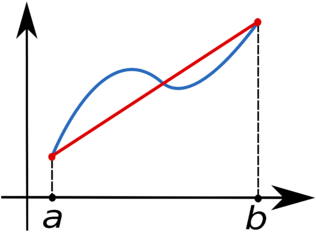
$$ \int_{a}^{b}f(x)dx $$we can partition the integration interval $[a,b]$ into smaller subintervals, and approximate the area under the curve for each subinterval by the area of the trapezoid created by linearly interpolating between the two function values at each end of the subinterval:
<img src="http://upload.wikimedia.org/wikipedia/commons/thumb/d/dd/Trapezoidal_rule_illustration.png/316px-Trapezoidal_rule_illustration.png" /img>
The blue line represents the function $f(x)$ and the red line is the linear interpolation. By subdividing the interval $[a,b]$, the area under $f(x)$ can thus be approximated as the sum of the areas of all the resulting trapezoids.
If we denote by $x_{i}$ ($i=0,\ldots,n,$ with $x_{0}=a$ and $x_{n}=b$) the abscissas where the function is sampled, then
$$ \int_{a}^{b}f(x)dx\approx\frac{1}{2}\sum_{i=1}^{n}\left(x_{i}-x_{i-1}\right)\left(f(x_{i})+f(x_{i-1})\right). $$The common case of using equally spaced abscissas with spacing $h=(b-a)/n$ reads simply
$$ \int_{a}^{b}f(x)dx\approx\frac{h}{2}\sum_{i=1}^{n}\left(f(x_{i})+f(x_{i-1})\right). $$One frequently receives the function values already precomputed, $y_{i}=f(x_{i}),$ so the equation above becomes
$$ \int_{a}^{b}f(x)dx\approx\frac{1}{2}\sum_{i=1}^{n}\left(x_{i}-x_{i-1}\right)\left(y_{i}+y_{i-1}\right). $$
In [ ]:
In [ ]:
In [ ]:
In [ ]: