Assignment 1.

Formalia:

Please read the assignment overview page carefully before proceeding. This page contains information about formatting (including formats etc), group sizes, and many other aspects of handing in the assignment.

If you fail to follow these simple instructions, it will negatively impact your grade!

Due date and time: The assignment is due on Sunday Februrary 28th, 2016 at 23:55. Hand in your IPython notebook file (with extension .ipynb) via http://peergrade.io.

Peergrading date and time: Remember that after handing in you have 24 hours to evaluate a few assignments written by other members of the class. Thus, the peer evaluations are due on Monday February 29th, 2016 at 23:55.

Assignment 1A: Anscombe's quartet

Start by downloading these four datasets: Data 1, Data 2, Data 3, and Data 4. The format is .tsv, which stands for tab separated values. Each file has two columns (separated using the tab character). The first column is $x$-values, and the second column is $y$-values.

It's ok to just download these files to disk by right-clicking on each one, but if you use Python and urllib or urllib2 to get them, I'll really be impressed. If you don't know how to do that, I recommend opening up Google and typing "download file using Python" or something like that. When interpreting the search results remember that stackoverflow is your friend.

• Using the numpy function mean, calculate the mean of both $x$-values and $y$-values for each dataset.
• Use python string formatting to print precisely two decimal places of these results to the output cell. Check out this stackoverflow page for help with the string formatting.
• Now calculate the variance for all of the various sets of $x$- and $y$-values (to three decimal places).
• Use numpy to calculate the Pearson correlation between $x$- and $y$-values for all four data sets (also to three decimal places).
• The next step is use linear regression to fit a straight line $f(x) = a x + b$ through each dataset and report $a$ and $b$ (to two decimal places). An easy way to fit a straight line in Python is using scipy's linregress. It works like this

  from scipy import stats
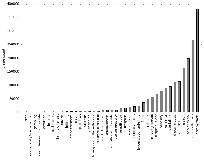
  slope, intercept, r_value, p_value, std_err = stats.linregress(x,y)

• Finally, it's time to plot the four datasets using matplotlib.pyplot. Use a two-by-two subplot to put all of the plots nicely in a grid and use the same $x$ and $y$ range for all four plots. And include the linear fit in all four plots. (To get a sense of what I think the plot should look like, you can take a look at my version here.)
• Explain - in your own words - what you think my point with this exercise is.

Assignment 1B: Slicing data

We investigate the types of crime and how they take place across San Francisco's police districts.

• We'll be combining information about PdDistrict and Category to explore differences between SF's neighborhoods. First, simply list the names of SF's 10 police districts.
• Which has the most crimes? Which has the most focus crimes?
• Next, we want to generate a slightly more complicated graphic. I'm interested to know if there are certain crimes that happen much more in certain neighborhoods than what's typical. Below I describe how to get that plot going
  • First, we need to calculate the relative probabilities of seeing each type of crime in the dataset as a whole. That's simply a normalized version of this plot. Let's call it P(crime).
  • Next, we calculate that same probability distribution but for each PD district, let's call that P(crime|district).
  • Now we look at the ratio P(crime|district)/P(crime). That ratio is equal to 1 if the crime occurs at the same level within a district as in the city as a whole. If it's greater than one, it means that the crime occurs more frequently within that district. If it's smaller than one, it means that the crime is rarer within the district in question than in the city as a whole.
  • For each district plot these ratios for the 14 focus crimes. My plot looks like this
  • Comment on the top crimes in Tenderloin, Mission, and Richmond. Does this fit with the impression you get of these neighborhoods on Wikipedia?
  • Even though we only plotted the ratios for our 14 focus crimes, I asked you to calculate the ratios based on all crime categories. Why do you think I wanted to include all crime types in the calculation?

Assignment 1C: KNN

The goal of this exercise is to create a useful real-world version of the example on pp153 in DSFS. We know from last week's exercises that the focus crimes PROSTITUTION, DRUG/NARCOTIC and DRIVING UNDER THE INFLUENCE tend to be concentrated in certain neighborhoods, so we focus on those crime types since they will make the most sense a KNN - map.

• Begin by using geoplotlib to plot all incidents of the three crime types on their own map using geoplotlib.kde(). This will give you an idea of how the varioius crimes are distributed across the city.
• Next, it's time to set up your model based on the actual data. You can use the code supplied in the book or try out scikit-learn's KNeighborsClassifier. If you end up using the latter (recommended), you may want to check out this example to get a sense of the usage.
  • You don't have to think a lot about testing/trainig and accuracy for this exercise. We're mostly interested in creating a map that's not too problematic. But do calculate the number of observations of each crime-type respectively. You'll find that the levels of each crime varies (lots of drug arrests, an intermediate amount of prostitiution registered, and very little drunk driving in the dataset). Since the algorithm classifies each point according to it's neighbors, what could a consequence of this imbalance in the number of examples from each class mean for your map?
  • You can make the dataset 'balanced' by grabbing an equal number of examples from each crime category. How do you expect that will change the KNN result? In which situations is the balanced map useful - and when is the map that data in proportion to occurrences useful? Choose which map you will work on in the following.
• Now create an approximately square grid of point that runs over SF. You get to decide the grid-size, but I recommend somewhere between $50 \times 50$ and $100 \times 100$ points. I recommend plotting using geoplotlib.dot().
• Visualize your model by coloring the grid, coloring each grid point according to it's category. Create a plot of this kind for models where each point is colored according to the majority of its 5, 10, and 30 nearest neighbors. Describe what happens to the map as you increase the number of neighbors, K.

Assignment 1D: Multiple regression and the Red Baron

Investigate Chief Suneman's idea is that the Red Baron might pick the time of his attacks according to a pattern that we can detect using the powers of data science.

If he's right, we can identify the time of the next attack, which will help us end this insanity once and for all. Well, let's see if he is right!

• Start from all cases having Red Baron in the resolution field and use the day of the week to predict the hour of the day when he is attacking, e.g. use linear regression to infer the hour of the day based on the weekday! Again, take 4/5 of the data for training and then calculate goodness of fit using $R^2$ on the rest 1/5. Don't forget to rescale your input variables! (Note 1: My goodness of fit after using the weekdays is only around 0.618). (Note 2: For multivariate regression, as always you can simply re-use the code in the DSFS book (Chapters 14-15) or scikit-learn).
• Now, add the crime year as well to the input variables! Did the goodness of fit improve? (Note: Mine did to 0.809)
• It is still low. Inspired by a movie he once watched, Chief Suneman yells: "Let's add the longitude of the crimes as well!" Is your prediction getting better? (It should, to around 0.993)
• Very nice! Why not add latitude as well? What do you find now?