In the Github repository you will find all you need to finish this workshop https://github.com/drabastomek/bigdl-fun.git:
Grab the jar from the jars folder appropriate for your version of Spark.
Similarly to uploading the BigDL upload the data from the data folder. Upload the data into the /tmp folder in your default storage.
First, let's configure our session.
In [1]:


%%configure -f
{
    "jars": ["wasb:///bigdl-0.2.0-SNAPSHOT-spark-2.0-jar-with-dependencies.jar"],

     "conf":{
         "spark.executorEnv.DL_ENGINE_TYPE": "mklblas",
         "spark.executorEnv.MKL_DISABLE_FAST_MM": "1",
         "spark.executorEnv.KMP_BLOCKTIME": "0",
         "spark.executorEnv.OMP_WAIT_POLICY": "passive",
         "spark.executorEnv.OMP_NUM_THREADS":"1",
         "spark.yarn.appMasterEnv.DL_ENGINE_TYPE": "mklblas",
         "spark.yarn.appMasterEnv.MKL_DISABLE_FAST_MM": "1",
         "spark.yarn.appMasterEnv.KMP_BLOCKTIME": "0",
         "spark.yarn.appMasterEnv.OMP_WAIT_POLICY": "passive",
         "spark.yarn.appMasterEnv.OMP_NUM_THREADS": "1"
     }
}
First, we load the BigDL jar from the Azure Blob Storage account. Please, make sure you adapted it to your version of Spark! We're using Spark 2.0 in this notebook.
Second, we specify additional environment variables required for the BigDL to work:
"passive" makes threads passive i.e. the threads do not consume processor cycles while waitingSpecifying the spark.executorEnv.<environment variable> sets the environment variables on the executors, whereas setting the spark.yarn.appMasterEnv.<environment variable> creates the variables on the head (driver) node; the latter is necessarily set this way as Jupyter runs in a yarn-cluster mode: check http://spark.apache.org/docs/latest/submitting-applications.html#launching-applications-with-spark-submit for more details about the differences between the client and cluster modes.
In [2]:


import com.intel.analytics.bigdl.utils.Engine

val nodeNumber = 2
val coreNumber = 8
val mult = 64
val batchSize = nodeNumber * coreNumber * mult

Engine.init(nodeNumber, coreNumber, true)
We will use two nodes with eight cores each. The batchSize will be later used to split the data into a set of mini batches. Running the Engine.init(...) sets several parameters for the BigDL engine to work; each executor will run a multi-threaded operation doing the processing of the data.
In [3]:
import com.intel.analytics.bigdl._
import com.intel.analytics.bigdl.numeric.NumericFloat
import com.intel.analytics.bigdl.nn._
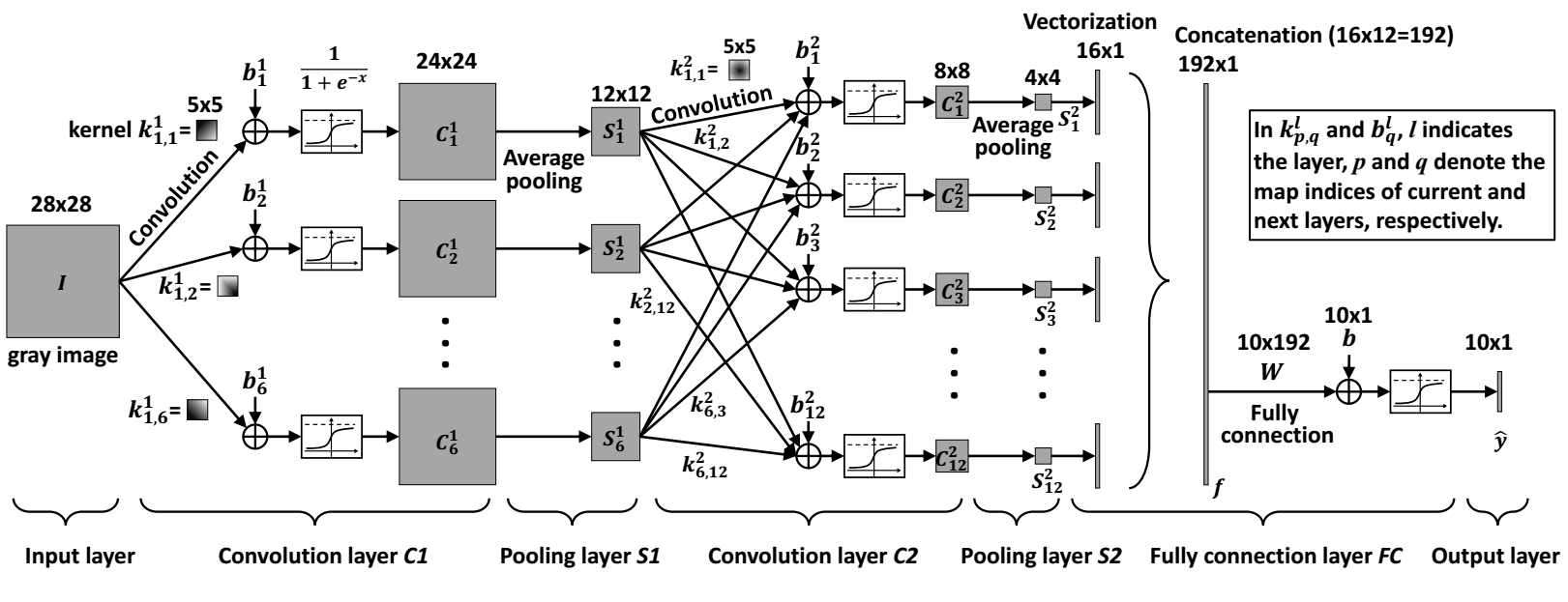
def buildModel(classNum: Int): Module[Float] = {
val model = Sequential()
model
.add(Reshape(Array(1, 28, 28)))
.add(SpatialConvolution(1, 6, 5, 5).setName("conv1_5x5"))
.add(Tanh())
.add(SpatialMaxPooling(2, 2, 2, 2))
.add(Tanh())
.add(SpatialConvolution(6, 12, 5, 5).setName("conv2_5x5"))
.add(SpatialMaxPooling(2, 2, 2, 2))
.add(Reshape(Array(12 * 4 * 4)))
.add(Linear(12 * 4 * 4, 100).setName("fc1"))
.add(Tanh())
.add(Linear(100, classNum).setName("fc2"))
.add(LogSoftMax())
}
Overall, there are 7 layers in our network:
Let's see how these are implemented by analyzing the code above:
Reshape(...) method: it takes an image as a input and reshapes the input image to 28x28 matrix (in case it was of a different size).SpatialConvolution(...). The first parameter is the number of input dimensions (in our case 1 as we process grey images, we'd set it to 3 if we used RGB colors). We will output 6 planes that measure 24x24 (Why? Tip: 5x5 and the 28x28 size of the input.) What we are training in this part of the network is the kernel structure. The last two parameters specify size of the kernel (note: the kernels should have odd-numbered dimensions e.g. 3x3 or 7x7 -- why?). The outputs from the kernels are then squashed using the Tanh() function so the values are in the $<-1; 1>$ range.SpatialMaxPooling(...) method. The pooling scans through the outputs of the convolutional layer 1 and averages the output given the kernel size. The first two parameters specify the kernel width and height, the remaining two specify the horizontal and vertical step size. The outputs from this layer are again squashed using the Tanh() function.Linear(...) layer that uses a linear function $y=Wx+b$ ($W$ stands for the matrix of weights and $b$ is bias). The layer takes the 192 element output from the pooling layer and outputs a 100 values that are being once again squashed by the Tanh() function. The last linear layer reduces the number of outputs to 10 - the number of the digits we try to recognize. LogSoftMax() layer assigns the digit probability to the input by using the following formula $$y_i=\log\Bigg(\frac{\exp(x_{i})}{\sum_{j}\exp(x_{j})}\Bigg)$$
In [4]:


import java.nio.ByteBuffer
import java.nio.file.Path
import com.intel.analytics.bigdl.dataset._
import com.intel.analytics.bigdl.dataset.image._
import com.intel.analytics.bigdl.models.lenet.Utils

def loadBinaryFile(filePath: Path): Array[Byte] = {
    val files = sc.binaryFiles(filePath.toString())
    val bytes = files.first()._2.toArray()
    bytes
}
The LoadBinaryFile(...) takes filePath as input and returns an array of bytes. Since the files are stream of binary data we treat them as such when reading them in into Spark.
In [5]:


def load(featureFile: Path, labelFile: Path): Array[ByteRecord] = {
    // read the data in
    val labelBuffer = ByteBuffer.wrap(loadBinaryFile(labelFile))
    val featureBuffer = ByteBuffer.wrap(loadBinaryFile(featureFile))

    // check the magic numbers
    val labelMagicNumber = labelBuffer.getInt()
    require(labelMagicNumber == 2049)

    val featureMagicNumber = featureBuffer.getInt()
    require(featureMagicNumber == 2051)

    // check if the counts agree between images and labels files
    val labelCount = labelBuffer.getInt()
    val featureCount = featureBuffer.getInt()
    require(labelCount == featureCount)

    // get number of columns and rows per image
    val rowNum = featureBuffer.getInt()
    val colNum = featureBuffer.getInt()

    // output buffer
    val result = new Array[ByteRecord](featureCount)

    var i = 0
    while (i < featureCount) {
        // new image
        val img = new Array[Byte]((rowNum * colNum))

        var y = 0
        while (y < rowNum) {
            var x = 0
            while (x < colNum) {
                // put the read pixel information in the right position
                img(x + y * colNum) = featureBuffer.get()
                x += 1
            }
            y += 1
        }

        // append to results as ByteRecord (add label)
        result(i) = ByteRecord(img, labelBuffer.get().toFloat + 1.0f)
        i += 1
  }
  result
}
The load(...) method requires two parameters: the paths to featureFile and labelFile; it returns an array of ByteRecords. The ByteRecord is a wrapper around an Array of bytes with an added label https://github.com/intel-analytics/BigDL/blob/master/spark/dl/src/main/scala/com/intel/analytics/bigdl/dataset/Types.scala.
The format of the datasets can be found on http://yann.lecun.com/exdb/mnist/ but here it is in a nutshell:
LABEL FILES:

[offset] [type]          [value]          [description]
0000     32 bit integer  0x00000801(2049) magic number (MSB first)
0004     32 bit integer  60000            number of items
0008     unsigned byte   ??               label
0009     unsigned byte   ??               label
........
xxxx     unsigned byte   ??               label
The labels values are 0 to 9.

TRAINING FILES:

[offset] [type]          [value]          [description]
0000     32 bit integer  0x00000803(2051) magic number
0004     32 bit integer  60000            number of images
0008     32 bit integer  28               number of rows
0012     32 bit integer  28               number of columns
0016     unsigned byte   ??               pixel
0017     unsigned byte   ??               pixel
........
xxxx     unsigned byte   ??               pixel
Given the above the flow of the function should now be self-explanatory.
Next, we specify the locations of the files.
In [6]:


val dir = "/tmp"

val trainDataFile = "train-images-idx3-ubyte"
val trainLabelFile = "train-labels-idx1-ubyte"
val validationDataFile = "t10k-images-idx3-ubyte"
val validationLabelFile = "t10k-labels-idx1-ubyte"
And read the files.
In [7]:


import java.nio.file.Paths
import com.intel.analytics.bigdl.DataSet
import com.intel.analytics.bigdl.dataset._
import com.intel.analytics.bigdl.dataset.image._

val trainData = Paths.get(dir, trainDataFile)
val trainLabel = Paths.get(dir, trainLabelFile)
val validationData = Paths.get(dir, validationDataFile)
val validationLabel = Paths.get(dir, validationLabelFile)

val trainMean = 0.13066047740239506
val trainStd = 0.3081078
val trainSet = {
    DataSet.array(load(trainData, trainLabel), sc) ->
    BytesToGreyImg(28, 28) ->
    GreyImgNormalizer(trainMean, trainStd) ->
    GreyImgToBatch(batchSize)
}

val testMean = 0.13251460696903547
val testStd = 0.31048024
val validationSet = {
    DataSet.array(load(validationData, validationLabel), sc) ->
    BytesToGreyImg(28, 28) ->
    GreyImgNormalizer(testMean, testStd) ->
    GreyImgToBatch(batchSize)
}
After reading the images using the load(...) method, we convert them to grey scale using the BytesToGreyImg(...) method. Using the GreyImgNormalizer(...) we normalize the image; this changes the range of pixel intensity (also know as contrast or histogram stretching). Lastly, we use the GreyImgToBatch(...) method to put the images into batches.
In [8]:


import com.intel.analytics.bigdl.nn._
import com.intel.analytics.bigdl.optim._
import com.intel.analytics.bigdl.utils._

// Train Lenet model
val initialModel = buildModel(10)  // 10 digit classes

val optimizer = Optimizer(
  model = initialModel,                   // training model
  dataset = trainSet,                     // training dataset
  criterion = ClassNLLCriterion[Float]()) // loss function
The initialModel object holds our model definition - we'll attempt to optimize it. The optimizer object is the optimization algorithm we'll use to train our network; we pass the initialModel as the model to be trained and our trainSet as the dataset to be learned from. The loss function chosen is the negative log-likelihood function - the ClassNLLCriterion[Float](); since the log-likelihood function is concave
and the optimizer's function is to minimize some cost-function we use the negative log-likelihood function
Check http://neuralnetworksanddeeplearning.com/chap3.html if you're interested in learning more about optimization.
Now it's time to optimize the model. We first set the learningRate and maxEpoch - the two hyperparameters of the network so we control the training rate and when we stop the training.
Setting the validation on the optimizer object instructs it to trigger the validation after eachEpoch using the validationSet (see https://stackoverflow.com/questions/2976452/whats-is-the-difference-between-train-validation-and-test-set-in-neural-networ): after each epoch the top1Accuracy is checked to control for the overfitting. We stop the training after 15 epochs. Finally, we call the optimize() method that triggerst the training process to start.
In [9]:


// Set hyperparameters. we set learningrate and max epochs
val state = T("learningRate" -> 0.05 / 4 * mult)

// Set maximum epochs
val maxEpoch = 15

val trainedModel = {optimizer.setValidation(
        trigger = Trigger.everyEpoch,
        dataset = validationSet,
        vMethods = Array(new Top1Accuracy)
    ).setState(state)
    .setEndWhen(Trigger.maxEpoch(maxEpoch))
    .optimize()
}
Once the training is done (normally it would take ~2-3 minutes) we can check how well we've done.
Let's see: using the Validator and the trainedModel we can test the accuracy of the model on the validationSet. Calling the .test(...) method on the validator will trigger the network to process the validation data and produce the output that is then compared to the original (expected) labels.
In [10]:


// import com.intel.analytics.bigdl.optim.{LocalValidator, Top1Accuracy, Validator}

val validator = Validator(trainedModel, validationSet)
val result = validator.test(Array(new Top1Accuracy[Float]))

result.foreach(r => {
  println(s"${r._2} is ${r._1}")
})
As you can we we got a respectable 99% accuracy; if you are willing to let it train for more than 15 epochs the accuracy should increase but be careful not to overfit your model.
Neural networks are well known for solving some of the most complex problems we currently encounter. Here are some interesting resouces for you to browse through: