Describing and implementing multivariate linear regression in Julia.
Definitions:
Let the set of $m$ training examples be $T = \{(\vec{x_{i}}, y_i)\}$ for $0 \leq i \leq m - 1$
where $\vec{x_{i}} \in \mathbb{R}^n$ is the $i^\text{th}$ training example input, and $n$ is the number of features, $y_i \in \mathbb{R}$ is $i^\text{th}$ is the training output.
Let $x_{i,j}$ denote the $j^\text{th}$ feature of the $i^\text{th}$ training example.
The linear regression hypothesis function $h_\vec{\theta} : \mathbb{R}^n \rightarrow \mathbb{R}$ has form:
$$h_\vec{\theta}(\vec{x}) = \sum_{i=0}^{n} \theta_{i} x_{i} = \vec{\theta}^{T} \vec{x}$$
Where we take $x_0 = 1$, and let $\vec{\theta} \in \mathbb{R}^{n+1}$ be the parameter vector.
The cost function $J : \mathbb{R}^{n+1} \rightarrow \mathbb{R}$ has form:
$$J(\vec{\theta}) = \frac{1}{2 m}\sum_{i=1}^{m}(h_\vec{\theta}(\vec{x}_{i}) - y_i)^2 = \frac{1}{2 m}\sum_{i=1}^{m}(\vec{\theta}^{T} \vec{x} - y_i)^2$$
We want to minimize the cost function $J$ by varying the parameter vector $\vec{\theta}$.
In this case, we can analytically solve this problem by solving the system of equations for $(\theta_0, \theta_1, \dotsc, \theta_{n})^T$ given by $\frac{\partial}{\partial \theta_i}{J(\vec{\theta})} = 0$ for all $i \in \{0,1,...,n\}$.
We can alternatively use an optimization algorithm like gradient descent, and we can recycle it for other min/max problems; so I'll go over that.
One method to find the parameter vector is the gradient descent algorithm.
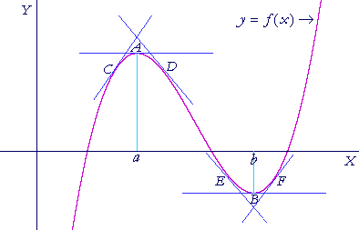
The idea in gradient descent is similar to the idea in single variable calculus:
Where we know that $\frac{d}{dx} f(x) = 0$ at the extrema (points A and B), and $\frac{d}{dx} f(x)$ can otherwise be used direct us toward the nearest (local) minimum/maximum (e.g. the slope of the lines at points C, D, E, F).
For a multivariate function $f : \mathbb{R}^n \rightarrow \mathbb{R}$, we use the vector differential, or gradient: $\vec{\nabla} f(x)$ to guide us to a minimum.
(Mnemonic side note: the latin root "gradi" means "to walk"--with the gradient we walk uphill at the steepest grade.)
For example, in:
A gradient vector field is shown projected beneath a plot of the function $f(x,y) = −(\cos^2 x + \cos^2 y)^2.$
Note that the vectors are pointed to the direction of maximum ascent--i.e. away from the minimum, thus if we want to minimize our cost function $J$ in the linear regression problem, we need to look toward the opposite direction: $-\vec{\nabla} f(x)$.
To see how we actually follow that direction, consider the Taylor expansion of $f(\vec{x}_0 + h\vec{\epsilon})$ where $\epsilon \in \mathbb{R}^{n+1}$ is a unit-vector that we want to minimize in the direction of if we start at vector $\vec{x}_0$, and $h \in \mathbb{R}$ is a constant "step-size":
$$
f(\vec{x}_0 + h\vec{\epsilon}) = f(\vec{x}_0) + h\vec{\nabla} f(\vec{x}_0) \cdot \vec{\epsilon} + h^2\text{(const. error)}
$$
If we take $h$ to be very small such that $h^2$ is even smaller, then let's regard $h^2\text{(const. error)} \approx 0$ so that:
$$
f(\vec{x}_0 + h\vec{\epsilon}) \approx f(\vec{x}_0) + h\vec{\nabla} f(\vec{x}_0) \cdot \vec{\epsilon}
$$
We want to choose a vector $\vec{\epsilon}$ that minimizes $f(\vec{x}_0 + h\vec{\epsilon})$.
i.e. that minimizes
$f(\vec{x}_0) + h\vec{\nabla} f(\vec{x}_0) \cdot \vec{\epsilon}$.
Note that $\vec{\nabla} f(\vec{x}_0) \cdot \vec{\epsilon} = \lvert \vec{\nabla} f(\vec{x}_0) \rvert \lvert \vec{\epsilon} \rvert \cos \delta$ where $\delta$ is the angle between $\vec{\nabla} f(\vec{x}_0)$ and $\vec{\epsilon}$.
By choosing unit-vector $\vec{\epsilon} = \frac{-\vec{\nabla} f(\vec{x}_0)}{\lvert \vec{\nabla} f(\vec{x}_0) \rvert}$, we have $\cos(\delta) = -1$, its least value.
So taking:
$\vec{x_1} = \vec{x}_0 + h\vec{\epsilon} = \vec{x}_0 - h\vec{\nabla} f(\vec{x}_0)$ for some step-size $h$,
and inspecting whether $f(\vec{x_{i+1}}) - f(\vec{x_{i}})$ reaches convergence within some threshold, we have the basic gradient descent algorithm.
To implement it with our cost function, we need the $i^\text{th}$ component of $\vec{\nabla}J(\vec{\theta})$.
This is given by: $\frac{\partial}{\partial \theta_i} J(\vec{\theta}) = \frac{1}{m} \sum_{j=1}^{m}x_{j,i}(\vec{\theta}^T \cdot \vec{x}_j - y_j)$
Julia has "metaprogramming" support: http://docs.julialang.org/en/latest/manual/metaprogramming/
The DataFrames package provides a "Formula" object for use in regression modeling: DataFrames.Formula
The syntax of formulae seems similar to that of R formulae, which is in turn derived from the "S" language:
Chambers and Hastie (1993) "Statistical Models in S" is the definitive reference for formulas in S and thus R, although their conception of formulas has been extended for other uses, and there is a package "formula" that defines a new object class Formula that inherits from class formula. At the R command line, ?formula will give you some details.
The design notes describe the language of the formulas:
Design Notes
And we can just look at the source: https://github.com/JuliaStats/DataFrames.jl/blob/master/src/formula.jl
In [1]:


using DataFrames
using RDatasets

iris = data("datasets", "iris")
# The DataFrames formula parser seems to take issue with column names having periods
# and I don't know if there's some proper way to escape them--so I'll just rename them:
# Uses string.replace: https://github.com/JuliaLang/julia/blob/master/base/string.jl
# and dataframe.rename: https://github.com/JuliaStats/DataFrames.jl/blob/master/src/dataframe.jl
#
# Also note that we need to use "rename!" to operate in place.
for col_name in DataFrames.colnames(iris)
    DataFrames.rename!(iris, col_name, replace(col_name, "\.", "_"))
end

print(head(iris))
In [1]:


# Suppose we want to predict petal width as a function of sepal.length, sepal.width, and petal.length
# for the "setosa" species.
# data_set = iris[:(Species .== "setosa"), :][["Sepal.Length", "Sepal.Width", "Petal.Length", "Petal.Width"]]
mf = ModelFrame(Formula(:(Petal_Width ~ Sepal_Length + Sepal_Width + Petal_Length)),
                iris[:(Species .== "setosa"), :])
mm = ModelMatrix(mf);
In [2]:


using DataFrames
using RDatasets
using PyPlot
In [3]:


# Parameters:
#    training_data is a DataFrames.DataFrame (https://github.com/JuliaStats/DataFrames.jl/blob/master/src/dataframe.jl)
#    containing the training data.
#
#    reg_formula is a DataFrames.Formula (https://github.com/JuliaStats/DataFrames.jl/blob/master/src/formula.jl)
#    specifying the linear equation to be fitted from training data.
#
# Example:
#
function linreg(training_data::DataFrame, reg_formula::Formula,
                step_size::Float64, threshold::Float64, max_iter::Float64)
    mf = ModelFrame(reg_formula, training_data)
    mm = ModelMatrix(mf) # mm.m is the matrix data with constant-param 1 column added.

    # Size of training set
    m = size(training_data,1)
    # Number of features
    n = size(mm, 2)

    # Column vector:
    theta = zeros(Float64, n, 1)

    # Hypothesis fcn: (theta_0' * mm.m[i,:])
    # x_i vector: mm.m[i,:]
    # y vector: model_response(mf)
    iter_cnt = 0
    diff = 1
    while diff > threshold && iter_cnt < max_iter
        # grad = (theta dot x_i - y_i)*x_i
        grad = [(sum([theta[j]*(mm.m[i,j]) for j=1:n]) - model_response(mf)[i])*mm.m[i,:] for i=1:m]
        theta1 = theta - (step_size/m)*sum(grad)'
        diff = sqrt(sum([x^2 for x in theta1 - theta]))
        theta = theta1
        iter_cnt += 1
        if iter_cnt % 3000 == 0
            println(("itercnt", iter_cnt))
            println(theta)
        end
    end

    println(("itercnt", iter_cnt))
    println(theta)

    return theta
end
Out[3]:
Let's try it out:
In [4]:


# Get some test data:
iris_test = data("datasets", "iris")
for col_name in DataFrames.colnames(iris)
    DataFrames.rename!(iris_test, col_name, replace(col_name, "\.", "_"))
end

# 2D test on iris data:
p = linreg(iris[:(Species .== "setosa"), :],
           Formula(:(Petal_Width ~ Sepal_Length)),
           0.075,
           1e-6,
           1e7)
Out[4]:
Let's plot what we got:
In [5]:


n = length(iris[:(Species .== "setosa"), :]["Sepal_Length"])

PyPlot.plt.clf()
PyPlot.plot(iris[:(Species .== "setosa"), :]["Sepal_Length"],
            iris[:(Species .== "setosa"), :]["Petal_Width"],
            "k.")

t = PyPlot.linspace(3, 6, n)
PyPlot.plot(t, p[1] + p[2]*t, "g.-")
#PyPlot.plot(t, t1 + t0*t, "b.-")
plt.gcf()
Out[5]:
Let's compare it to some existing library:
In [6]:


using PyCall
@pyimport numpy

n = length(iris[:(Species .== "setosa"), :]["Sepal_Length"])

PyPlot.plt.clf()
PyPlot.plot(iris[:(Species .== "setosa"), :]["Sepal_Length"],
            iris[:(Species .== "setosa"), :]["Petal_Width"],
            "k.")
(t0,t1) = numpy.polyfit(iris[:(Species .== "setosa"), :]["Sepal_Length"],
                        iris[:(Species .== "setosa"), :]["Petal_Width"],
                        1)

t = PyPlot.linspace(3, 6, n)
PyPlot.plot(t, t1 + t0*t, "b.-")
plt.gcf()
Out[6]:
Let's try it in 3d.
In [7]:


# Get some test data:
iris_test = data("datasets", "iris")
for col_name in DataFrames.colnames(iris)
    DataFrames.rename!(iris_test, col_name, replace(col_name, "\.", "_"))
end

# 2D test on iris data:
p = linreg(iris[:(Species .== "setosa"), :],
           Formula(:(Petal_Width ~ Sepal_Length + Petal_Length)),
           0.035,
           1e-6,
           1e7)

# Not quite sure how best to 3d plot in Julia.
# Matplotlib has a mplot3d package, but I couldn't quickly get it going:
#@pyimport mpl_toolkits
#fig = plt.gcf()
#ax = fig.add_subplot(111, projection="3d")
#
# There's also "gaston": https://github.com/mbaz/Gaston.jl
# which is a front-end for gnuplot, which is 3d capable.
Out[7]: