Before we get started on today's main topics, we want to close off last week's discussion on regression by addressing some common methods that improve the results given by the standard linear regression model.
Think back to the regression models we studied last week, where we generated new features in order to model a nonlinear relationship between inputs and outputs. With more features, our predictive models were able to recognize more of the underlying relationships.
However, consider a problem where we are predicting with a large amount of features in the input space relative to the amount of data that we have. While the inputs and outputs of our training set may be related by an underlying function, there will also be noise in the training data, and working with too many possible features can cause the model to overfit the data by learning the noise.
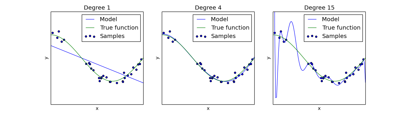
http://scikit-learn.org/0.15/_images/plot_underfitting_overfitting_0011.png
In the plots above, the plot on the left illustrates underfitting (by using only one feature in the polynomial regression), while the one on the right illustrates overfitting (by using 15 features that causes the model to fit a 15 degree polynomial).
Ridge regression is motivated by the idea that we can prevent overfitting by limiting the sum of the weights of the model. Intuitively, by limiting the coefficients of the regression, ridge regression causes only the most relevant features to be represented. This reduces the problem of overfitting while still allowing for the flexibility a large feature space.
$$ \sum (y_i - \sum_{j=0}^{p}B_j x_{ij})^2 + \lambda \sum_{j=0}^{p}B_j^2 $$The first term is the same as in Ordinary Least Squares. The second term penalizes large coefficient. The effect is to "shrink" the coefficients that result from minimizing the cost function.
One potential drawback to ridge regression is that the coefficients can be made very small, but never zero. Many datasets have a sparse feature space - there can be many features, but only a few have relevant predictive power. In these cases, we want to allow some coefficients to be 0, representing that they are not relevant to the prediction in any way. Ridge regression may cause these coefficients to have very small values, but Lasso regression allows these coefficients to go to 0 - this doesn't dramatically improve predictive power over the lasso regression, but it makes it much cleaner to see what features actually contributed to the prediction.
$$\sum (y_i - \sum_{j=0}^{p}B_j x_{ij})^2 + \lambda \sum_{j=0}^{p}|{B_j}| $$This is the same as Ridge Regression but instead of penalizing the squares of the coefficients we penalize the absolute value of the coefficients. Feel free to read more about why this leads to some coefficients being set to 0, but we're not going to go over it here, since the mathematics is somewhat complicated. The advantage of this approach is that we simultaneously perform variable selection, which leads to more interpretable results.
Regularization is important, as overfitting is one of the main problems that plagues vanilla linear regression. Regularization maintains the flexibility of large feature spaces while ensuring that the large feature spaces aren't too sensitive to noise. The tuning parameter controls the sensitivity of the model to noise, and this can be tuned using cross validation to find the optimal values for the data set.
Ridge regression ensures small coefficients, while Lasso regression further ensures that coefficients can be zeroed out. There exist many other regularization methods out there. For example, elastic net regression is a hybrid model that combines the error terms for Ridge and Lasso regression.
For this workshop's challenge, go to the Scikit-learn documentation to figure out how to use their Ridge and Lasso implementations. You'll be comparing how the regularized regressions perform relative to standard linear regression.
In [28]:


from sklearn.datasets import load_boston
from sklearn.cross_validation import train_test_split
from sklearn import linear_model

boston = load_boston()
x_train, x_test, y_train, y_test = train_test_split(boston.data, boston.target, test_size=0.15)
First, see how normal regression fits
In [ ]:


# TODO: run standard linear regression, print coefficients and mean squared error
Now, model a Ridge regression on the same dataset and compare the results by looking at the mean squared error
In [29]:


# TODO: run ridge regression, print coefficients and mean squared error
Finally, model a Lasso regression on the same dataset, compare the coefficients and MSE with the Ridge model.
In [30]:


# TODO: run lasso regression, print coefficients and mean squared error