Class, Race, and Sex in Virginia Criminal Courts

This notebook is supplemental material for a blog post I wrote (i.e., Uncovering Big Bias with Big Data). If you haven't read it, please take a moment and start there.

If you're new to notebooks, check out this quick start guide. Also, I've tried to provide useful links for people new to this sort of thing throughout.

UPDATE: The Lawyerist piece was written as a vehicle for introducing attorneys to regression analysis. Consequently, I made modeling choices informed by an attempt to maximize ease of understanding on the part of my audience while minimizing complaints from experts. As you can imagine, that's a hard balance. The overwhelming majority of comments and critiques were thoughtful, and most of them quite correct as suggestions for improving the model's predictive power. A sampling of the most frequent include: Why didn't you treat seriousness levels as categorical variables? What about collinearity? Shouldn't you include defendants' past criminal history? You call that cross-validation?

Fair or not, transparency (in the form of this notebook) was my primary relief value, inviting others to pick up where I left off and improve on the model. There's a reason I made such a fuss in the piece about the model not being a good predictive model, and why I pushed the George Box quote so hard. In short, the complexity that full examinations of the above and similar suggestions would have added to the piece would have likely lost my intended audience, and I'm not convinced such additional detail would have added much for said audience. At it's heart, the model presented is a discussion starter, "It’s important to note what we’re doing is modeling for insight. I don’t expect that we’ll use our model to predict the future. Rather, we’re trying to figure out how things interact. We want to know what happens to outcomes when we vary defendant demographics, specifically their race or income. The exact numbers aren’t as important as the general trends and how they compare... there’s a lot more one could do with this data..."

That being said, my hope is to find the time to revisit this dataset with an eye towards a different audience. Namely, one that will allow me to further explore the nuances in the data and address the issues raised by those readers looking for more robust analysis.

Load Modules

These are libraries we'll need to conduct our analysis.


In [1]:
import matplotlib.pyplot as plt
%matplotlib inline
import numpy as np
import pandas as pd
import seaborn as sns
from statsmodels.formula.api import ols
import statsmodels.api as sm
from IPython.display import Image

Data Wrangling & Exploration

All of our court data will be coming from here: VA Court Data, maintained by Ben Schoenfeld (@oilytheotter). As the blog post makes clear, we'll be restricting our analysis to 2006-2010. So we'll start by loading data for that timeframe.

FYI, you'll notice that I'm referencing a directory not contained in this repo (i.e., ../data/). I did this so I don't have to worry about any of the issues that come with hosting such data in a publicly accessable repository. See note on data privacy.


In [2]:
# read in data
list_ = []
i = 0
yr = 2006
while yr <= 2010:
    k = 0
    while k < 12:
        k += 1  
        #print ("loading: ../data/criminal_circuit_court_cases_%s/criminal_circuit_court_cases_%s_%s.csv"%(yr,yr,k))
        list_.append(pd.read_csv("../data/criminal_circuit_court_cases_%s/criminal_circuit_court_cases_%s_%s.csv"%(yr,yr,k), low_memory=False))
        i += 1  
    yr += 1  
charges_df = pd.concat(list_)

# display first 4 rows
# charges_df[:4]

The reason we're focused on 2006-2010 is that we can use defendant zip codes to join our court data with American Community Survey (ACS) data on income. So below we'll pull out defendant zip codes and place them in their own column. To do this we use some magic known as regular expressions.


In [3]:
# Pull out zipcode to match with census data 
charges_df['Zip'] = charges_df['Address'].str.extract('([0-9]*$)', expand=False)
# drop charges where zip can't be found
charges_df = charges_df[pd.notnull(charges_df['Zip'])]
# Make sure the zip is a number
charges_df['Zip'] = pd.to_numeric(charges_df['Zip'])
# fill in NaN (blank cells) to ease later work
charges_df = charges_df.fillna(value="")
# print new count

So now we need that income data. I found a nice spreadsheet with it over here: Zip Code Characteristics. Note the file MedianZIP-3.xlsx actually contained both mean and media values. Anywho, I downloaded the spreadsheet and saved it as a .csv called zip_income.csv. Then I cleaned it up a bit.


In [4]:
# Load the csv file into a dataframe
zip_df = pd.read_csv("../data/zip_income.csv") 
# There were commas in the data. So let's strip those out. 
zip_df['Median'] = zip_df['Median'].str.replace(',', '')
zip_df['Mean'] = zip_df['Mean'].str.replace(',', '')
# Also, we won't need the population column. So let's drop that too.
zip_df = zip_df.drop('Pop', 1)
# Exclude zip codes not in VA see http://www.zipcodestogo.com/Virginia/
zip_df = zip_df[zip_df['Zip']>=20101]
zip_df = zip_df[zip_df['Zip']!=23909] # note there was an error in this entry so I had to remove it
zip_df = zip_df[zip_df['Zip']<=26886]
zip_df['Mean'] = pd.to_numeric(zip_df['Mean'])
zip_df['Median'] = pd.to_numeric(zip_df['Median'])
# display first 4 rows
zip_df[:4]


Out[4]:
Zip Median Mean
6027 20105 136228 163021
6028 20106 73043 91799
6029 20109 66077 75929
6030 20110 79914 91429

So now we need to construct some features. Again, the blog post has more context. Note, here are some explinations of charge types: Virginia Misdemeanor Crimes by Class and Sentences and Virginia Felony Crimes by Class and Sentences. Also, if you're unfamiliar with the idea of joins here's a primer with visuals. It's talking about SQL, but the concept holds.


In [11]:
# merge original data set and ACS data. THis is a join
munged_df = pd.merge(charges_df,zip_df,how='inner',on='Zip')

#
# NOTE: THE ORIGINAL VERSION OF THIS NOTEBOOK NEGLECTED TO REMOVE ENTERIES 
# WITH UNIDENTIFIED RACE AND SEX COLUMNS. THE FOLLOWING LINES CORRECT THIS.
#
munged_df = munged_df[munged_df['Race'] != '']
munged_df = munged_df[munged_df['Sex'] != '']

# Translate charge types into positions on an ordered list from 1 and 10 
munged_df['Seriousness'] = 0
munged_df.loc[(munged_df['ChargeType'].str.contains('Misdemeanor',case=False)==True) & (munged_df['Class'].str.contains('1',case=False)==True), 'Seriousness'] = 4
munged_df.loc[(munged_df['ChargeType'].str.contains('Misdemeanor',case=False)==True) & (munged_df['Class'].str.contains('2',case=False)==True), 'Seriousness'] = 3
munged_df.loc[(munged_df['ChargeType'].str.contains('Misdemeanor',case=False)==True) & (munged_df['Class'].str.contains('3',case=False)==True), 'Seriousness'] = 2
munged_df.loc[(munged_df['ChargeType'].str.contains('Misdemeanor',case=False)==True) & (munged_df['Class'].str.contains('4',case=False)==True), 'Seriousness'] = 1
munged_df.loc[(munged_df['ChargeType'].str.contains('Felony',case=False)==True) & (munged_df['Class'].str.contains('1',case=False)==True), 'Seriousness'] = 10
munged_df.loc[(munged_df['ChargeType'].str.contains('Felony',case=False)==True) & (munged_df['Class'].str.contains('2',case=False)==True), 'Seriousness'] = 9
munged_df.loc[(munged_df['ChargeType'].str.contains('Felony',case=False)==True) & (munged_df['Class'].str.contains('3',case=False)==True), 'Seriousness'] = 8
munged_df.loc[(munged_df['ChargeType'].str.contains('Felony',case=False)==True) & (munged_df['Class'].str.contains('4',case=False)==True), 'Seriousness'] = 7
munged_df.loc[(munged_df['ChargeType'].str.contains('Felony',case=False)==True) & (munged_df['Class'].str.contains('5',case=False)==True), 'Seriousness'] = 6
munged_df.loc[(munged_df['ChargeType'].str.contains('Felony',case=False)==True) & (munged_df['Class'].str.contains('6',case=False)==True), 'Seriousness'] = 5
munged_df = munged_df[munged_df['Seriousness'] > 0]

# Break out each race category so they can be considered by the linear regression
munged_df['Male'] = 0
munged_df.loc[munged_df['Sex'] == 'Male', 'Male'] = 1
munged_df['Native'] = 0
munged_df.loc[munged_df['Race'].str.contains('american',case=False)==True, 'Native'] = 1
munged_df['Asian'] = 0
munged_df.loc[munged_df['Race'].str.contains('asian',case=False)==True, 'Asian'] = 1
munged_df['Black'] = 0
munged_df.loc[munged_df['Race'].str.contains('black',case=False)==True, 'Black'] = 1
munged_df['Hispanic'] = 0
munged_df.loc[munged_df['Race'] == 'Hispanic', 'Hispanic'] = 1
munged_df['Other'] = 0
munged_df.loc[munged_df['Race'].str.contains('other',case=False)==True, 'Other'] = 1

# figure out what our sentece should be. Note: originally I was dooing more than renaming. So this is really some vestigle code. 
munged_df['SentenceDays'] = pd.to_numeric(munged_df['SentenceTimeDays'])
munged_df['SentenceDays_T'] = np.log(1+munged_df['SentenceDays'])
munged_df = munged_df.fillna(value=0)

# partition data for cross-validation
holdout = munged_df.sample(frac=0.2)
training = munged_df.loc[~munged_df.index.isin(holdout.index)]

# optional print to file
munged_df.to_csv(path_or_buf='../data/output.csv')

#output_sample = munged_df[(munged_df['Seriousness'] <= 2) & (munged_df['SentenceDays'] > 0)]
#output_sample = munged_df.sample(n=5000)
#output_sample.to_csv(path_or_buf='../data/output_sample.csv')

# display first four rows
munged_df[:4]


Out[11]:
AKA AKA2 Address AmendedCharge AmendedChargeType AmendedCodeSection ArrestDate CaseNumber Charge ChargeType ... Mean Seriousness Male Native Asian Black Hispanic Other SentenceDays SentenceDays_T
0 TOPPING, VA 23169 DIST.MARIJ.<1/2 OZ. Misdemeanor 18.2-248.1 10/25/2005 CR04003010-01 DIST.MARIJUANA Felony ... 57734 6 1 0 1 0 0 0 365.0 5.902633
8 TOPPING, VA 23169 02/27/2005 CR05000044-00 DRIVING INTOXICATED Misdemeanor ... 57734 4 1 0 1 0 0 0 0.0 0.000000
9 TOPPING, VA 23169 06/22/2005 CR05000106-00 POSS. FIREARM BY FELON Felony ... 57734 5 1 0 1 0 0 0 1825.0 7.509883
11 TOPPING, VA 23169 CR06000069-00 RECKLESS DRIVING 84/65 MPH Misdemeanor ... 57734 4 1 0 1 0 0 0 0.0 0.000000

4 rows × 59 columns

Analysis

If you're not familiar with linear regressions, read the blog post then check out this: Introduction to Linear Regression.


In [6]:
# Run a simple linear regression & print the P values
model = ols("SentenceDays ~ Seriousness", training).fit()
print("P-values:\n%s"%model.pvalues)

# Plot regression
fig = sns.lmplot(x="Seriousness", y="SentenceDays", data=munged_df, scatter_kws={"s": 20, "alpha": 0.25}, order=1)
plt.rc('font', family='serif', monospace='Courier') # http://matplotlib.org/users/usetex.html
plt.title("Linear Regression\n(All Data Points)",  fontsize = 17, y=1.05)
plt.xlabel('Seriousness')
plt.ylabel('Sentence in Days')
plt.annotate('R-squared: %f'%(model.rsquared), (0,0), (0,-45),  fontsize = 11, xycoords='axes fraction', textcoords='offset points', va='top')
plt.savefig('../data/tmp/f1.1.png',bbox_inches='tight');


P-values:
Intercept      0.0
Seriousness    0.0
dtype: float64

In [9]:
# Run a simple linear regression & print the P values
model = ols("SentenceDays ~ Seriousness", training).fit()
print("P-values:\n%s"%model.pvalues)

# Plot Regression with estimator
fig = sns.lmplot(x="Seriousness", y="SentenceDays", data=munged_df, x_estimator=np.mean, order=1)
plt.rc('font', family='serif', monospace='Courier') #http://matplotlib.org/users/usetex.html
plt.title("Linear Regression\n(Representative \"Dots\")",  fontsize = 17, y=1.05)
plt.xlabel('Seriousness')
plt.ylabel('Sentence in Days')
plt.annotate('R-squared: %f'%(model.rsquared), (0,0), (0,-45), fontsize = 11, xycoords='axes fraction', textcoords='offset points', va='top')
plt.savefig('../data/tmp/f1.2.png',bbox_inches='tight');


P-values:
Intercept      0.0
Seriousness    0.0
dtype: float64

In [9]:
# Run a simple linear regression & print the P values
model = ols("SentenceDays ~ Seriousness + np.power(Seriousness, 2)", training).fit()
print("P-values:\n%s"%model.pvalues)

# Plot multiple subplot axes with seaborn
# h/t https://gist.github.com/JohnGriffiths/8605267
fig_outfile = '../data/tmp/fig_1.3.png'

# Plot the figs and save to temp files
fig = sns.lmplot(x="Seriousness", y="SentenceDays", data=munged_df, x_estimator=np.mean, order=2);
fig = (fig.set_axis_labels("Seriousness", "Sentence in Days"))
plt.suptitle("2nd Order Polynomial Regression\n(Representative \"Dots\")",  fontsize = 13, y=1.07)
plt.annotate('R-squared: %f'%(model.rsquared), (0,0), (0,-45), fontsize = 11, xycoords='axes fraction', textcoords='offset points', va='top')
plt.savefig('../data/tmp/f1.3.1.png',bbox_inches='tight'); plt.close()
model = ols("SentenceDays ~ Seriousness + np.power(Seriousness, 2) + np.power(Seriousness, 3)+ np.power(Seriousness, 4)", munged_df).fit()
print("P values:\n%s"%model.pvalues)
fig = sns.lmplot(x="Seriousness", y="SentenceDays", data=munged_df, x_estimator=np.mean, order=4);
fig = (fig.set_axis_labels("Seriousness", "Sentence in Days"))
plt.suptitle("4th Order Polynomial Regression\n(Representative \"Dots\")",  fontsize = 13, y=1.07)
plt.annotate('R-squared: %f'%(model.rsquared), (0,0), (0,-45), fontsize = 11, xycoords='axes fraction', textcoords='offset points', va='top')
plt.savefig('../data/tmp/f1.3.2.png',bbox_inches='tight'); plt.close()

# Combine them with imshows
fig, ax = plt.subplots(nrows=1, ncols=2, figsize=(12,6))
for a in [1,2]: ax[a-1].imshow(plt.imread('../data/tmp/f1.3.%s.png' %a)); ax[a-1].axis('off')
plt.tight_layout(); plt.savefig(fig_outfile,bbox_inches='tight'); plt.close() 

# Display in notebook as an image
Image(fig_outfile, width="100%")


P-values:
Intercept                    1.389605e-81
Seriousness                  3.977515e-32
np.power(Seriousness, 2)    2.806694e-110
dtype: float64
P values:
Intercept                   1.221946e-06
Seriousness                 9.431874e-06
np.power(Seriousness, 2)    5.982796e-09
np.power(Seriousness, 3)    3.620690e-23
np.power(Seriousness, 4)    1.048774e-34
dtype: float64
Out[9]:

In [10]:
# Run a simple linear regression & print the P values
model = ols("SentenceDays_T ~ Seriousness", training).fit()
print("P-values:\n%s"%model.pvalues)

# Plot multiple subplot axes with seaborn
# h/t https://gist.github.com/JohnGriffiths/8605267
fig_outfile = '../data/tmp/fig_2.png'

# Plot the figs and save to temp files
fig = sns.lmplot(x="Seriousness", y="SentenceDays_T", data=munged_df, scatter_kws={"s": 20, "alpha": 0.25}, order=1);
fig = (fig.set_axis_labels("Seriousness", "log(1 + Sentence in Days)"))
plt.suptitle("(All Data Points)",  fontsize = 14, y=1.03)
plt.savefig('../data/tmp/f2.1.png',bbox_inches='tight'); plt.close()
fig = sns.lmplot(x="Seriousness", y="SentenceDays_T", data=munged_df, x_estimator=np.mean, order=1);
fig = (fig.set_axis_labels("Seriousness", "log(1 + Sentence in Days)"))
plt.suptitle("(Representative \"Dots\")",  fontsize = 14, y=1.03)
plt.savefig('../data/tmp/f2.2.png',bbox_inches='tight'); plt.close()

# Combine them with imshows
fig, ax = plt.subplots(nrows=1, ncols=2, figsize=(12,6))
for a in [1,2]: ax[a-1].imshow(plt.imread('../data/tmp/f2.%s.png' %a)); ax[a-1].axis('off')
plt.suptitle("Log-Linear Regression",  fontsize = 17, y=1.02)
plt.tight_layout();
plt.annotate('R-squared: %f'%(model.rsquared), (-1.05,0), (0,-10), fontsize = 11, xycoords='axes fraction', textcoords='offset points', va='top')
plt.savefig(fig_outfile,bbox_inches='tight'); plt.close() 

# Display in notebook as an image
Image(fig_outfile, width="100%")


P-values:
Intercept      2.222211e-107
Seriousness     0.000000e+00
dtype: float64
Out[10]:

In [11]:
# Run a simple linear regression & print the P values
model = ols("SentenceDays_T ~ Seriousness + np.power(Seriousness, 2)", training).fit()
print("P-values:\n%s"%model.pvalues)

# Plot multiple subplot axes with seaborn
# h/t https://gist.github.com/JohnGriffiths/8605267
fig_outfile = '../data/tmp/fig_3.png'

# Plot the figs and save to temp files
fig = sns.lmplot(x="Seriousness", y="SentenceDays_T", data=munged_df, x_estimator=np.mean, order=2);
fig = (fig.set_axis_labels("Seriousness", "log(1 + Sentence in Days)"))
plt.suptitle("2nd Order Polynomial Regression\n(Representative \"Dots\")",  fontsize = 13, y=1.07)
plt.annotate('R-squared: %f'%(model.rsquared), (0,0), (0,-45),  fontsize = 11, xycoords='axes fraction', textcoords='offset points', va='top')
plt.savefig('../data/tmp/f3.1.png',bbox_inches='tight'); plt.close()
model = ols("SentenceDays_T ~ Seriousness + np.power(Seriousness, 2) + np.power(Seriousness, 3)+ np.power(Seriousness, 4)", munged_df).fit()
fig = sns.lmplot(x="Seriousness", y="SentenceDays_T", data=munged_df, x_estimator=np.mean, order=4);
fig = (fig.set_axis_labels("Seriousness", "log(1 + Sentence in Days)"))
plt.suptitle("4th Order Polynomial Regression\n(Representative \"Dots\")",  fontsize = 13, y=1.07)
plt.annotate('R-squared: %f'%(model.rsquared), (0,0), (0,-45),  fontsize = 11, xycoords='axes fraction', textcoords='offset points', va='top')
plt.savefig('../data/tmp/f3.2.png',bbox_inches='tight'); plt.close()

# Combine them with imshows
fig, ax = plt.subplots(nrows=1, ncols=2, figsize=(12,6))
for a in [1,2]: ax[a-1].imshow(plt.imread('../data/tmp/f3.%s.png' %a)); ax[a-1].axis('off')
plt.tight_layout(); plt.savefig(fig_outfile,bbox_inches='tight'); plt.close() 

# Display in notebook as an image
Image(fig_outfile, width="100%")


P-values:
Intercept                   0.0
Seriousness                 0.0
np.power(Seriousness, 2)    0.0
dtype: float64
Out[11]:

In [12]:
# Plot multiple linear regression 
# h/t https://www.datarobot.com/blog/multiple-regression-using-statsmodels/#appendix

from mpl_toolkits.mplot3d import Axes3D

X = training[['Seriousness', 'Mean']]
y = training['SentenceDays_T']

## fit a OLS model
X = sm.add_constant(X)
est = sm.OLS(y, X).fit()

## Create the 3d plot 
xx1, xx2 = np.meshgrid(np.linspace(X.Seriousness.min(), X.Seriousness.max(), 100), 
                       np.linspace(X.Mean.min(), X.Mean.max(), 100))

# plot the hyperplane by evaluating the parameters on the grid
Z = est.params[0] + est.params[1] * xx1 + est.params[2] * xx2

# create matplotlib 3d axes
fig = plt.figure(figsize=(12, 8))
ax = Axes3D(fig, azim=-120, elev=15)

# plot hyperplane
surf = ax.plot_surface(xx1, xx2, Z, cmap=plt.cm.RdBu_r, alpha=0.6, linewidth=0)

# plot data points
resid = y - est.predict(X)
ax.scatter(X[resid >= 0].Seriousness, X[resid >= 0].Mean, y[resid >= 0], color='black', alpha=0.25, facecolor='white')
ax.scatter(X[resid < 0].Seriousness, X[resid < 0].Mean, y[resid < 0], color='black', alpha=0.25)

# set axis labels
ax.set_title('Multiple Log-Linear Regression', fontsize = 20)
ax.set_xlabel('Seriousness')
ax.set_ylabel('Mean Income')
ax.set_zlabel('log(1 + Sentence in Days)')


Out[12]:
<matplotlib.text.Text at 0x143f6f8d0>

Cross Validation

So the code below doesn't really capture how I go about cross-validation, but as a supplement to the blog post, I wanted to provide a look at how one might compare multiple models. Below you'll see summary statistics from sets of different regressions run both on the training and holdout data. A good description of the summary statistics can be found in this article: Linear Regressuib with Python.

You'll also notice a graph associated with each regression. These are residual plots, and the folowing article should help you understand how to read them. Interpreting residual plots to improve your regression.


In [12]:
print("========================")
print("         LINEAR")
print("========================")
model = ols("SentenceDays ~ Seriousness + Male + Mean + Black + Hispanic + Asian + Native + Other", training).fit()
print(model.summary())
plt.scatter(model.fittedvalues,model.resid,alpha=0.25)
plt.xlabel('perdicted')
plt.ylabel('residuals')
plt.show()
model = ols("SentenceDays ~ Seriousness + Male + Mean + Black + Hispanic + Asian + Native + Other", holdout).fit()
print(model.summary())
plt.scatter(model.fittedvalues,model.resid,alpha=0.25)
plt.xlabel('perdicted')
plt.ylabel('residuals')
plt.show()

print("========================")
print("       2ND ORDER")
print("========================")
model = ols("SentenceDays ~ Seriousness + np.power(Seriousness, 2) + Male + Mean + Black + Hispanic + Asian + Native + Other", training).fit()
print(model.summary())
plt.scatter(model.fittedvalues,model.resid,alpha=0.25)
plt.xlabel('perdicted')
plt.ylabel('residuals')
plt.show()
model = ols("SentenceDays ~ Seriousness + np.power(Seriousness, 2) + Male + Mean + Black + Hispanic + Asian + Native + Other", holdout).fit()
print(model.summary())
plt.scatter(model.fittedvalues,model.resid,alpha=0.25)
plt.xlabel('perdicted')
plt.ylabel('residuals')
plt.show()

print("========================")
print("       4TH ORDER")
print("========================")
model = ols("SentenceDays ~ Seriousness + np.power(Seriousness, 2) + Male + Mean + Black + Hispanic + Asian + Native + Other", training).fit()
print(model.summary())
plt.scatter(model.fittedvalues,model.resid,alpha=0.25)
plt.xlabel('perdicted')
plt.ylabel('residuals')
plt.show()
model = ols("SentenceDays ~ Seriousness + np.power(Seriousness, 2) + Male + Mean + Black + Hispanic + Asian + Native + Other", holdout).fit()
print(model.summary())
plt.scatter(model.fittedvalues,model.resid,alpha=0.25)
plt.xlabel('perdicted')
plt.ylabel('residuals')
plt.show()

print("========================")
print("      LOG-LINEAR")
print("========================")
model = ols("np.log(1+SentenceDays) ~ Seriousness + Male + Mean + Black + Hispanic + Asian + Native + Other", training).fit()
print(model.summary())
plt.scatter(model.fittedvalues,model.resid,alpha=0.25)
plt.xlabel('perdicted')
plt.ylabel('residuals')
plt.show()
model = ols("np.log(1+SentenceDays) ~ Seriousness + Male + Mean + Black + Hispanic + Asian + Native + Other", holdout).fit()
print(model.summary())
plt.scatter(model.fittedvalues,model.resid,alpha=0.25)
plt.xlabel('perdicted')
plt.ylabel('residuals')
plt.show()

print("========================")
print("  2ND ORDER LOG-LINEAR")
print("========================")
model = ols("np.log(1+SentenceDays) ~ Seriousness + np.power(Seriousness, 2) + Male + Mean + Black + Hispanic + Asian + Native + Other", training).fit()
print(model.summary())
plt.scatter(model.fittedvalues,model.resid,alpha=0.25)
plt.xlabel('perdicted')
plt.ylabel('residuals')
plt.show()
model = ols("np.log(1+SentenceDays) ~ Seriousness + np.power(Seriousness, 2) + Male + Mean + Black + Hispanic + Asian + Native + Other", holdout).fit()
print(model.summary())
plt.scatter(model.fittedvalues,model.resid,alpha=0.25)
plt.xlabel('perdicted')
plt.ylabel('residuals')
plt.show()

print("========================")
print("  4TH ORDER LOG-LINEAR")
print("========================")
model = ols("np.log(1+SentenceDays) ~ Seriousness + np.power(Seriousness, 2) + Male + Mean + Black + Hispanic + Asian + Native + Other", training).fit()
print(model.summary())
plt.scatter(model.fittedvalues,model.resid,alpha=0.25)
plt.xlabel('perdicted')
plt.ylabel('residuals')
plt.show()
model = ols("np.log(1+SentenceDays) ~ Seriousness + np.power(Seriousness, 2) + Male + Mean + Black + Hispanic + Asian + Native + Other", holdout).fit()
print(model.summary())
plt.scatter(model.fittedvalues,model.resid,alpha=0.25)
plt.xlabel('perdicted')
plt.ylabel('residuals')
plt.show()


========================
         LINEAR
========================
                            OLS Regression Results                            
==============================================================================
Dep. Variable:           SentenceDays   R-squared:                       0.123
Model:                            OLS   Adj. R-squared:                  0.123
Method:                 Least Squares   F-statistic:                     3566.
Date:                Wed, 01 Jun 2016   Prob (F-statistic):               0.00
Time:                        03:00:08   Log-Likelihood:            -1.5121e+06
No. Observations:              177522   AIC:                         3.024e+06
Df Residuals:                  177514   BIC:                         3.024e+06
Df Model:                           7                                         
Covariance Type:            nonrobust                                         
===============================================================================
                  coef    std err          t      P>|t|      [95.0% Conf. Int.]
-------------------------------------------------------------------------------
Intercept    -958.7834     23.940    -40.049      0.000     -1005.706  -911.861
Seriousness   327.5419      2.136    153.355      0.000       323.356   331.728
Male          142.7949      6.538     21.842      0.000       129.981   155.608
Mean           -0.0010      0.000     -8.349      0.000        -0.001    -0.001
Black         -86.7664     21.029     -4.126      0.000      -127.982   -45.550
Hispanic     -164.4403     30.515     -5.389      0.000      -224.249  -104.632
Asian        -200.1446     20.878     -9.587      0.000      -241.064  -159.225
Native       -185.2072     93.692     -1.977      0.048      -368.841    -1.574
Other        -322.2249     41.093     -7.841      0.000      -402.766  -241.684
==============================================================================
Omnibus:                   256472.290   Durbin-Watson:                   1.563
Prob(Omnibus):                  0.000   Jarque-Bera (JB):        197843814.639
Skew:                           8.414   Prob(JB):                         0.00
Kurtosis:                     165.678   Cond. No.                     1.62e+19
==============================================================================

Warnings:
[1] Standard Errors assume that the covariance matrix of the errors is correctly specified.
[2] The smallest eigenvalue is 3.15e-24. This might indicate that there are
strong multicollinearity problems or that the design matrix is singular.
                            OLS Regression Results                            
==============================================================================
Dep. Variable:           SentenceDays   R-squared:                       0.128
Model:                            OLS   Adj. R-squared:                  0.128
Method:                 Least Squares   F-statistic:                     927.7
Date:                Wed, 01 Jun 2016   Prob (F-statistic):               0.00
Time:                        03:00:09   Log-Likelihood:            -3.7958e+05
No. Observations:               44380   AIC:                         7.592e+05
Df Residuals:                   44372   BIC:                         7.593e+05
Df Model:                           7                                         
Covariance Type:            nonrobust                                         
===============================================================================
                  coef    std err          t      P>|t|      [95.0% Conf. Int.]
-------------------------------------------------------------------------------
Intercept    -994.0340     53.050    -18.738      0.000     -1098.013  -890.055
Seriousness   345.6603      4.441     77.835      0.000       336.956   354.365
Male          143.7682     13.494     10.654      0.000       117.320   170.217
Mean           -0.0010      0.000     -3.914      0.000        -0.001    -0.000
Black        -127.5577     47.444     -2.689      0.007      -220.549   -34.567
Hispanic     -240.8303     67.239     -3.582      0.000      -372.620  -109.041
Asian        -264.2061     47.148     -5.604      0.000      -356.618  -171.794
Native         45.7721    214.233      0.214      0.831      -374.127   465.672
Other        -407.2120     89.581     -4.546      0.000      -582.791  -231.633
==============================================================================
Omnibus:                    65749.842   Durbin-Watson:                   1.983
Prob(Omnibus):                  0.000   Jarque-Bera (JB):         54023172.866
Skew:                           8.830   Prob(JB):                         0.00
Kurtosis:                     173.009   Cond. No.                     1.41e+20
==============================================================================

Warnings:
[1] Standard Errors assume that the covariance matrix of the errors is correctly specified.
[2] The smallest eigenvalue is 1.05e-26. This might indicate that there are
strong multicollinearity problems or that the design matrix is singular.
========================
       2ND ORDER
========================
                            OLS Regression Results                            
==============================================================================
Dep. Variable:           SentenceDays   R-squared:                       0.125
Model:                            OLS   Adj. R-squared:                  0.125
Method:                 Least Squares   F-statistic:                     3169.
Date:                Wed, 01 Jun 2016   Prob (F-statistic):               0.00
Time:                        03:00:10   Log-Likelihood:            -1.5119e+06
No. Observations:              177522   AIC:                         3.024e+06
Df Residuals:                  177513   BIC:                         3.024e+06
Df Model:                           8                                         
Covariance Type:            nonrobust                                         
============================================================================================
                               coef    std err          t      P>|t|      [95.0% Conf. Int.]
--------------------------------------------------------------------------------------------
Intercept                 -557.4091     32.233    -17.293      0.000      -620.586  -494.232
Seriousness                147.9848      9.900     14.949      0.000       128.582   167.388
np.power(Seriousness, 2)    15.9851      0.861     18.574      0.000        14.298    17.672
Male                       136.6068      6.540     20.889      0.000       123.789   149.425
Mean                        -0.0011      0.000     -9.280      0.000        -0.001    -0.001
Black                       -6.4542     21.449     -0.301      0.763       -48.493    35.585
Hispanic                   -92.2676     30.732     -3.002      0.003      -152.502   -32.034
Asian                     -114.9383     21.356     -5.382      0.000      -156.795   -73.081
Native                     -95.4472     93.726     -1.018      0.309      -279.148    88.253
Other                     -248.3017     41.245     -6.020      0.000      -329.142  -167.462
==============================================================================
Omnibus:                   253999.266   Durbin-Watson:                   1.561
Prob(Omnibus):                  0.000   Jarque-Bera (JB):        190779060.592
Skew:                           8.256   Prob(JB):                         0.00
Kurtosis:                     162.749   Cond. No.                     2.32e+19
==============================================================================

Warnings:
[1] Standard Errors assume that the covariance matrix of the errors is correctly specified.
[2] The smallest eigenvalue is 1.54e-24. This might indicate that there are
strong multicollinearity problems or that the design matrix is singular.
                            OLS Regression Results                            
==============================================================================
Dep. Variable:           SentenceDays   R-squared:                       0.132
Model:                            OLS   Adj. R-squared:                  0.132
Method:                 Least Squares   F-statistic:                     844.6
Date:                Wed, 01 Jun 2016   Prob (F-statistic):               0.00
Time:                        03:00:12   Log-Likelihood:            -3.7947e+05
No. Observations:               44380   AIC:                         7.590e+05
Df Residuals:                   44371   BIC:                         7.590e+05
Df Model:                           8                                         
Covariance Type:            nonrobust                                         
============================================================================================
                               coef    std err          t      P>|t|      [95.0% Conf. Int.]
--------------------------------------------------------------------------------------------
Intercept                 -321.7939     69.057     -4.660      0.000      -457.148  -186.440
Seriousness                 42.4854     20.497      2.073      0.038         2.312    82.659
np.power(Seriousness, 2)    27.1276      1.791     15.150      0.000        23.618    30.637
Male                       131.4621     13.484      9.750      0.000       105.033   157.891
Mean                        -0.0012      0.000     -4.618      0.000        -0.002    -0.001
Black                        9.8665     48.184      0.205      0.838       -84.575   104.308
Hispanic                  -121.3349     67.529     -1.797      0.072      -253.692    11.023
Asian                     -118.2022     48.005     -2.462      0.014      -212.293   -24.112
Native                     179.5993    213.866      0.840      0.401      -239.581   598.780
Other                     -271.7226     89.797     -3.026      0.002      -447.727   -95.718
==============================================================================
Omnibus:                    64563.752   Durbin-Watson:                   1.984
Prob(Omnibus):                  0.000   Jarque-Bera (JB):         50144686.833
Skew:                           8.521   Prob(JB):                         0.00
Kurtosis:                     166.790   Cond. No.                     9.74e+19
==============================================================================

Warnings:
[1] Standard Errors assume that the covariance matrix of the errors is correctly specified.
[2] The smallest eigenvalue is 2.19e-26. This might indicate that there are
strong multicollinearity problems or that the design matrix is singular.
========================
       4TH ORDER
========================
                            OLS Regression Results                            
==============================================================================
Dep. Variable:           SentenceDays   R-squared:                       0.125
Model:                            OLS   Adj. R-squared:                  0.125
Method:                 Least Squares   F-statistic:                     3169.
Date:                Wed, 01 Jun 2016   Prob (F-statistic):               0.00
Time:                        03:00:13   Log-Likelihood:            -1.5119e+06
No. Observations:              177522   AIC:                         3.024e+06
Df Residuals:                  177513   BIC:                         3.024e+06
Df Model:                           8                                         
Covariance Type:            nonrobust                                         
============================================================================================
                               coef    std err          t      P>|t|      [95.0% Conf. Int.]
--------------------------------------------------------------------------------------------
Intercept                 -557.4091     32.233    -17.293      0.000      -620.586  -494.232
Seriousness                147.9848      9.900     14.949      0.000       128.582   167.388
np.power(Seriousness, 2)    15.9851      0.861     18.574      0.000        14.298    17.672
Male                       136.6068      6.540     20.889      0.000       123.789   149.425
Mean                        -0.0011      0.000     -9.280      0.000        -0.001    -0.001
Black                       -6.4542     21.449     -0.301      0.763       -48.493    35.585
Hispanic                   -92.2676     30.732     -3.002      0.003      -152.502   -32.034
Asian                     -114.9383     21.356     -5.382      0.000      -156.795   -73.081
Native                     -95.4472     93.726     -1.018      0.309      -279.148    88.253
Other                     -248.3017     41.245     -6.020      0.000      -329.142  -167.462
==============================================================================
Omnibus:                   253999.266   Durbin-Watson:                   1.561
Prob(Omnibus):                  0.000   Jarque-Bera (JB):        190779060.592
Skew:                           8.256   Prob(JB):                         0.00
Kurtosis:                     162.749   Cond. No.                     2.32e+19
==============================================================================

Warnings:
[1] Standard Errors assume that the covariance matrix of the errors is correctly specified.
[2] The smallest eigenvalue is 1.54e-24. This might indicate that there are
strong multicollinearity problems or that the design matrix is singular.
                            OLS Regression Results                            
==============================================================================
Dep. Variable:           SentenceDays   R-squared:                       0.132
Model:                            OLS   Adj. R-squared:                  0.132
Method:                 Least Squares   F-statistic:                     844.6
Date:                Wed, 01 Jun 2016   Prob (F-statistic):               0.00
Time:                        03:00:14   Log-Likelihood:            -3.7947e+05
No. Observations:               44380   AIC:                         7.590e+05
Df Residuals:                   44371   BIC:                         7.590e+05
Df Model:                           8                                         
Covariance Type:            nonrobust                                         
============================================================================================
                               coef    std err          t      P>|t|      [95.0% Conf. Int.]
--------------------------------------------------------------------------------------------
Intercept                 -321.7939     69.057     -4.660      0.000      -457.148  -186.440
Seriousness                 42.4854     20.497      2.073      0.038         2.312    82.659
np.power(Seriousness, 2)    27.1276      1.791     15.150      0.000        23.618    30.637
Male                       131.4621     13.484      9.750      0.000       105.033   157.891
Mean                        -0.0012      0.000     -4.618      0.000        -0.002    -0.001
Black                        9.8665     48.184      0.205      0.838       -84.575   104.308
Hispanic                  -121.3349     67.529     -1.797      0.072      -253.692    11.023
Asian                     -118.2022     48.005     -2.462      0.014      -212.293   -24.112
Native                     179.5993    213.866      0.840      0.401      -239.581   598.780
Other                     -271.7226     89.797     -3.026      0.002      -447.727   -95.718
==============================================================================
Omnibus:                    64563.752   Durbin-Watson:                   1.984
Prob(Omnibus):                  0.000   Jarque-Bera (JB):         50144686.833
Skew:                           8.521   Prob(JB):                         0.00
Kurtosis:                     166.790   Cond. No.                     9.74e+19
==============================================================================

Warnings:
[1] Standard Errors assume that the covariance matrix of the errors is correctly specified.
[2] The smallest eigenvalue is 2.19e-26. This might indicate that there are
strong multicollinearity problems or that the design matrix is singular.
========================
      LOG-LINEAR
========================
                               OLS Regression Results                               
====================================================================================
Dep. Variable:     np.log(1 + SentenceDays)   R-squared:                       0.060
Model:                                  OLS   Adj. R-squared:                  0.060
Method:                       Least Squares   F-statistic:                     1615.
Date:                      Wed, 01 Jun 2016   Prob (F-statistic):               0.00
Time:                              03:00:15   Log-Likelihood:            -4.5707e+05
No. Observations:                    177522   AIC:                         9.141e+05
Df Residuals:                        177514   BIC:                         9.142e+05
Df Model:                                 7                                         
Covariance Type:                  nonrobust                                         
===============================================================================
                  coef    std err          t      P>|t|      [95.0% Conf. Int.]
-------------------------------------------------------------------------------
Intercept       0.4915      0.063      7.823      0.000         0.368     0.615
Seriousness     0.5672      0.006    101.186      0.000         0.556     0.578
Male            0.3350      0.017     19.523      0.000         0.301     0.369
Mean        -4.251e-06   3.18e-07    -13.385      0.000     -4.87e-06 -3.63e-06
Black           0.3692      0.055      6.690      0.000         0.261     0.477
Hispanic        0.3887      0.080      4.854      0.000         0.232     0.546
Asian           0.1891      0.055      3.451      0.001         0.082     0.296
Native          0.3726      0.246      1.516      0.130        -0.109     0.855
Other          -0.8282      0.108     -7.679      0.000        -1.040    -0.617
==============================================================================
Omnibus:                     1656.478   Durbin-Watson:                   1.431
Prob(Omnibus):                  0.000   Jarque-Bera (JB):            20782.384
Skew:                          -0.240   Prob(JB):                         0.00
Kurtosis:                       1.394   Cond. No.                     1.62e+19
==============================================================================

Warnings:
[1] Standard Errors assume that the covariance matrix of the errors is correctly specified.
[2] The smallest eigenvalue is 3.15e-24. This might indicate that there are
strong multicollinearity problems or that the design matrix is singular.
                               OLS Regression Results                               
====================================================================================
Dep. Variable:     np.log(1 + SentenceDays)   R-squared:                       0.058
Model:                                  OLS   Adj. R-squared:                  0.058
Method:                       Least Squares   F-statistic:                     393.5
Date:                      Wed, 01 Jun 2016   Prob (F-statistic):               0.00
Time:                              03:00:17   Log-Likelihood:            -1.1432e+05
No. Observations:                     44380   AIC:                         2.287e+05
Df Residuals:                         44372   BIC:                         2.287e+05
Df Model:                                 7                                         
Covariance Type:                  nonrobust                                         
===============================================================================
                  coef    std err          t      P>|t|      [95.0% Conf. Int.]
-------------------------------------------------------------------------------
Intercept       0.5339      0.135      3.968      0.000         0.270     0.798
Seriousness     0.5604      0.011     49.759      0.000         0.538     0.582
Male            0.2974      0.034      8.690      0.000         0.230     0.364
Mean        -3.838e-06   6.33e-07     -6.065      0.000     -5.08e-06  -2.6e-06
Black           0.4025      0.120      3.345      0.001         0.167     0.638
Hispanic        0.2663      0.171      1.562      0.118        -0.068     0.600
Asian           0.1700      0.120      1.422      0.155        -0.064     0.404
Native          0.4664      0.543      0.858      0.391        -0.598     1.531
Other          -0.7712      0.227     -3.395      0.001        -1.217    -0.326
==============================================================================
Omnibus:                      428.508   Durbin-Watson:                   1.987
Prob(Omnibus):                  0.000   Jarque-Bera (JB):             5233.903
Skew:                          -0.244   Prob(JB):                         0.00
Kurtosis:                       1.390   Cond. No.                     1.41e+20
==============================================================================

Warnings:
[1] Standard Errors assume that the covariance matrix of the errors is correctly specified.
[2] The smallest eigenvalue is 1.05e-26. This might indicate that there are
strong multicollinearity problems or that the design matrix is singular.
========================
  2ND ORDER LOG-LINEAR
========================
                               OLS Regression Results                               
====================================================================================
Dep. Variable:     np.log(1 + SentenceDays)   R-squared:                       0.080
Model:                                  OLS   Adj. R-squared:                  0.080
Method:                       Least Squares   F-statistic:                     1935.
Date:                      Wed, 01 Jun 2016   Prob (F-statistic):               0.00
Time:                              03:00:18   Log-Likelihood:            -4.5513e+05
No. Observations:                    177522   AIC:                         9.103e+05
Df Residuals:                        177513   BIC:                         9.104e+05
Df Model:                                 8                                         
Covariance Type:                  nonrobust                                         
============================================================================================
                               coef    std err          t      P>|t|      [95.0% Conf. Int.]
--------------------------------------------------------------------------------------------
Intercept                   -3.0259      0.084    -36.127      0.000        -3.190    -2.862
Seriousness                  2.1407      0.026     83.220      0.000         2.090     2.191
np.power(Seriousness, 2)    -0.1401      0.002    -62.643      0.000        -0.144    -0.136
Male                         0.3892      0.017     22.903      0.000         0.356     0.422
Mean                      -3.26e-06   3.14e-07    -10.366      0.000     -3.88e-06 -2.64e-06
Black                       -0.3346      0.056     -6.003      0.000        -0.444    -0.225
Hispanic                    -0.2437      0.080     -3.052      0.002        -0.400    -0.087
Asian                       -0.5576      0.055    -10.048      0.000        -0.666    -0.449
Native                      -0.4140      0.244     -1.700      0.089        -0.891     0.063
Other                       -1.4760      0.107    -13.772      0.000        -1.686    -1.266
==============================================================================
Omnibus:                     2272.788   Durbin-Watson:                   1.425
Prob(Omnibus):                  0.000   Jarque-Bera (JB):            21780.606
Skew:                          -0.282   Prob(JB):                         0.00
Kurtosis:                       1.380   Cond. No.                     2.32e+19
==============================================================================

Warnings:
[1] Standard Errors assume that the covariance matrix of the errors is correctly specified.
[2] The smallest eigenvalue is 1.54e-24. This might indicate that there are
strong multicollinearity problems or that the design matrix is singular.
                               OLS Regression Results                               
====================================================================================
Dep. Variable:     np.log(1 + SentenceDays)   R-squared:                       0.079
Model:                                  OLS   Adj. R-squared:                  0.079
Method:                       Least Squares   F-statistic:                     475.8
Date:                      Wed, 01 Jun 2016   Prob (F-statistic):               0.00
Time:                              03:00:19   Log-Likelihood:            -1.1383e+05
No. Observations:                     44380   AIC:                         2.277e+05
Df Residuals:                         44371   BIC:                         2.278e+05
Df Model:                                 8                                         
Covariance Type:                  nonrobust                                         
============================================================================================
                               coef    std err          t      P>|t|      [95.0% Conf. Int.]
--------------------------------------------------------------------------------------------
Intercept                   -2.9778      0.174    -17.148      0.000        -3.318    -2.637
Seriousness                  2.1442      0.052     41.600      0.000         2.043     2.245
np.power(Seriousness, 2)    -0.1417      0.005    -31.471      0.000        -0.151    -0.133
Male                         0.3617      0.034     10.667      0.000         0.295     0.428
Mean                     -2.929e-06   6.26e-07     -4.675      0.000     -4.16e-06  -1.7e-06
Black                       -0.3154      0.121     -2.603      0.009        -0.553    -0.078
Hispanic                    -0.3580      0.170     -2.108      0.035        -0.691    -0.025
Asian                       -0.5927      0.121     -4.910      0.000        -0.829    -0.356
Native                      -0.2327      0.538     -0.433      0.665        -1.287     0.821
Other                       -1.4790      0.226     -6.550      0.000        -1.922    -1.036
==============================================================================
Omnibus:                      570.969   Durbin-Watson:                   1.985
Prob(Omnibus):                  0.000   Jarque-Bera (JB):             5473.480
Skew:                          -0.283   Prob(JB):                         0.00
Kurtosis:                       1.375   Cond. No.                     9.74e+19
==============================================================================

Warnings:
[1] Standard Errors assume that the covariance matrix of the errors is correctly specified.
[2] The smallest eigenvalue is 2.19e-26. This might indicate that there are
strong multicollinearity problems or that the design matrix is singular.
========================
  4TH ORDER LOG-LINEAR
========================
                               OLS Regression Results                               
====================================================================================
Dep. Variable:     np.log(1 + SentenceDays)   R-squared:                       0.080
Model:                                  OLS   Adj. R-squared:                  0.080
Method:                       Least Squares   F-statistic:                     1935.
Date:                      Wed, 01 Jun 2016   Prob (F-statistic):               0.00
Time:                              03:00:20   Log-Likelihood:            -4.5513e+05
No. Observations:                    177522   AIC:                         9.103e+05
Df Residuals:                        177513   BIC:                         9.104e+05
Df Model:                                 8                                         
Covariance Type:                  nonrobust                                         
============================================================================================
                               coef    std err          t      P>|t|      [95.0% Conf. Int.]
--------------------------------------------------------------------------------------------
Intercept                   -3.0259      0.084    -36.127      0.000        -3.190    -2.862
Seriousness                  2.1407      0.026     83.220      0.000         2.090     2.191
np.power(Seriousness, 2)    -0.1401      0.002    -62.643      0.000        -0.144    -0.136
Male                         0.3892      0.017     22.903      0.000         0.356     0.422
Mean                      -3.26e-06   3.14e-07    -10.366      0.000     -3.88e-06 -2.64e-06
Black                       -0.3346      0.056     -6.003      0.000        -0.444    -0.225
Hispanic                    -0.2437      0.080     -3.052      0.002        -0.400    -0.087
Asian                       -0.5576      0.055    -10.048      0.000        -0.666    -0.449
Native                      -0.4140      0.244     -1.700      0.089        -0.891     0.063
Other                       -1.4760      0.107    -13.772      0.000        -1.686    -1.266
==============================================================================
Omnibus:                     2272.788   Durbin-Watson:                   1.425
Prob(Omnibus):                  0.000   Jarque-Bera (JB):            21780.606
Skew:                          -0.282   Prob(JB):                         0.00
Kurtosis:                       1.380   Cond. No.                     2.32e+19
==============================================================================

Warnings:
[1] Standard Errors assume that the covariance matrix of the errors is correctly specified.
[2] The smallest eigenvalue is 1.54e-24. This might indicate that there are
strong multicollinearity problems or that the design matrix is singular.
                               OLS Regression Results                               
====================================================================================
Dep. Variable:     np.log(1 + SentenceDays)   R-squared:                       0.079
Model:                                  OLS   Adj. R-squared:                  0.079
Method:                       Least Squares   F-statistic:                     475.8
Date:                      Wed, 01 Jun 2016   Prob (F-statistic):               0.00
Time:                              03:00:22   Log-Likelihood:            -1.1383e+05
No. Observations:                     44380   AIC:                         2.277e+05
Df Residuals:                         44371   BIC:                         2.278e+05
Df Model:                                 8                                         
Covariance Type:                  nonrobust                                         
============================================================================================
                               coef    std err          t      P>|t|      [95.0% Conf. Int.]
--------------------------------------------------------------------------------------------
Intercept                   -2.9778      0.174    -17.148      0.000        -3.318    -2.637
Seriousness                  2.1442      0.052     41.600      0.000         2.043     2.245
np.power(Seriousness, 2)    -0.1417      0.005    -31.471      0.000        -0.151    -0.133
Male                         0.3617      0.034     10.667      0.000         0.295     0.428
Mean                     -2.929e-06   6.26e-07     -4.675      0.000     -4.16e-06  -1.7e-06
Black                       -0.3154      0.121     -2.603      0.009        -0.553    -0.078
Hispanic                    -0.3580      0.170     -2.108      0.035        -0.691    -0.025
Asian                       -0.5927      0.121     -4.910      0.000        -0.829    -0.356
Native                      -0.2327      0.538     -0.433      0.665        -1.287     0.821
Other                       -1.4790      0.226     -6.550      0.000        -1.922    -1.036
==============================================================================
Omnibus:                      570.969   Durbin-Watson:                   1.985
Prob(Omnibus):                  0.000   Jarque-Bera (JB):             5473.480
Skew:                          -0.283   Prob(JB):                         0.00
Kurtosis:                       1.375   Cond. No.                     9.74e+19
==============================================================================

Warnings:
[1] Standard Errors assume that the covariance matrix of the errors is correctly specified.
[2] The smallest eigenvalue is 2.19e-26. This might indicate that there are
strong multicollinearity problems or that the design matrix is singular.

The Final Word

In the blog post I make use of a model to calculate how much money a person of color would need to earn in order to counteract race-base bias with class-based favor. The model below is the one I used. I opted to go with a log-linear model. This is in part because of its simplicity. As the post makes clear, I only need the model to be good enough to answer the question I'm asking (i.e., which is a bigger problem for the criminal justice system, race or class based bias?). And it has to be easily to explain the model to a general audience. That being said, this doesn't have to be the final word. Please take this work and expand on it. Just let me know how it goes.

Anywho, you'll notice that this model doesn't have the highest R-squared of the set. That's because I liked its residual plot better than the linear models with better R-squareds. As for the choice not to fit a polynomial, I didn't feel like I had very good theory to support such agressive fitting, and again, I'm just looking for an answer to my question, not a predictive model. That is, I'm modeling for insight. So I have a high tolerance for minor differences.

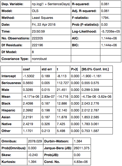
NOTE: an earlier version of this notebook neglected to remove enteries with unidentified race and sex. This issue has been corrected. However, it led the author to incorectly state the relative weights of the model's features. The corrected output is below. However, the old/incorrect summary statistics can still be found here and in this notebook's history.


In [15]:
model = ols("np.log(1+SentenceDays) ~ Seriousness + Male + Mean + Black + Hispanic + Asian + Native + Other", munged_df).fit()
#model = ols("np.log(1+SentenceDays) ~ Seriousness + Male + Mean + C(Race,Treatment(reference='White Caucasian (Non-Hispanic)'))", munged_df).fit()
model.summary()


Out[15]:
OLS Regression Results
Dep. Variable: np.log(1 + SentenceDays) R-squared: 0.060
Model: OLS Adj. R-squared: 0.060
Method: Least Squares F-statistic: 2008.
Date: Wed, 01 Jun 2016 Prob (F-statistic): 0.00
Time: 04:11:07 Log-Likelihood: -5.7139e+05
No. Observations: 221902 AIC: 1.143e+06
Df Residuals: 221894 BIC: 1.143e+06
Df Model: 7
Covariance Type: nonrobust
coef std err t P>|t| [95.0% Conf. Int.]
Intercept 0.4995 0.057 8.778 0.000 0.388 0.611
Seriousness 0.5659 0.005 112.764 0.000 0.556 0.576
Male 0.3273 0.015 21.341 0.000 0.297 0.357
Mean -4.166e-06 2.84e-07 -14.680 0.000 -4.72e-06 -3.61e-06
Black 0.3763 0.050 7.503 0.000 0.278 0.475
Hispanic 0.3660 0.072 5.051 0.000 0.224 0.508
Asian 0.1857 0.050 3.728 0.000 0.088 0.283
Native 0.3886 0.224 1.735 0.083 -0.050 0.828
Other -0.8171 0.097 -8.389 0.000 -1.008 -0.626
Omnibus: 2085.433 Durbin-Watson: 1.384
Prob(Omnibus): 0.000 Jarque-Bera (JB): 26018.148
Skew: -0.241 Prob(JB): 0.00
Kurtosis: 1.393 Cond. No. 1.93e+19

Here's the above model translated into an equation.

Note: if you're viewing this on GitHub, there seems to be a bug with thier equation formating. So if things look odd, that's why.

$$S=e^{\beta + \beta_1 x_1 + \beta_2 x_2 + \beta_3 x_3 + \beta_4 x_4 + \beta_5 x_5 + \beta_6 x_6 + \beta_7 x_7 + \beta_8 x_8 + \epsilon} \quad$$

Where:

  • D is our dataset of court cases joined with income data.
  • S is the Sentence in Days plus 1 day.
  • Coeficents β1 through β8 are those determined by an ordinary least squares (OLS) regression for the dataset D corresponding to features x1 through x8 repectivly, with β equal to the intercept. Values of these can be found in the table above along with P values and additional summary data. An explination of these summary statistics can be found here.
  • ε = some random error for the above OLS. See Forecasting From Log-Linear Regressions.
  • x1 = the seriousness level of a charge.
  • x2 = 1 if defendent is male, otherwise 0.
  • x3 = the mean income of the defendent's zip code.
  • x4 = 1 if defendent is Black, otherwise 0.
  • x5 = 1 if defendent is Hispanic, otherwise 0.
  • x6 = 1 if defendent is Asian, otherwise 0.
  • x7 = 1 if defendent is Native American, otherwise 0.
  • x8 = 1 if defendent is Other, otherwise 0.

For income’s influence to counteract that of being black $\beta_3 x_3 + \beta_3 x_4 = 0$

Therefore:

$$ –0.000004166x+(0.3763)(1)=0 $$$$ x=\frac{0.3763}{0.000004166} $$$$ x=\$90,326.45 $$

That is:

For a black man in a Virginia court to get the same treatment as his Caucasian peer, he needs to earn an additional $90,000 a year.

Similar amounts hold for American Indians and Hispanics.


In [ ]: